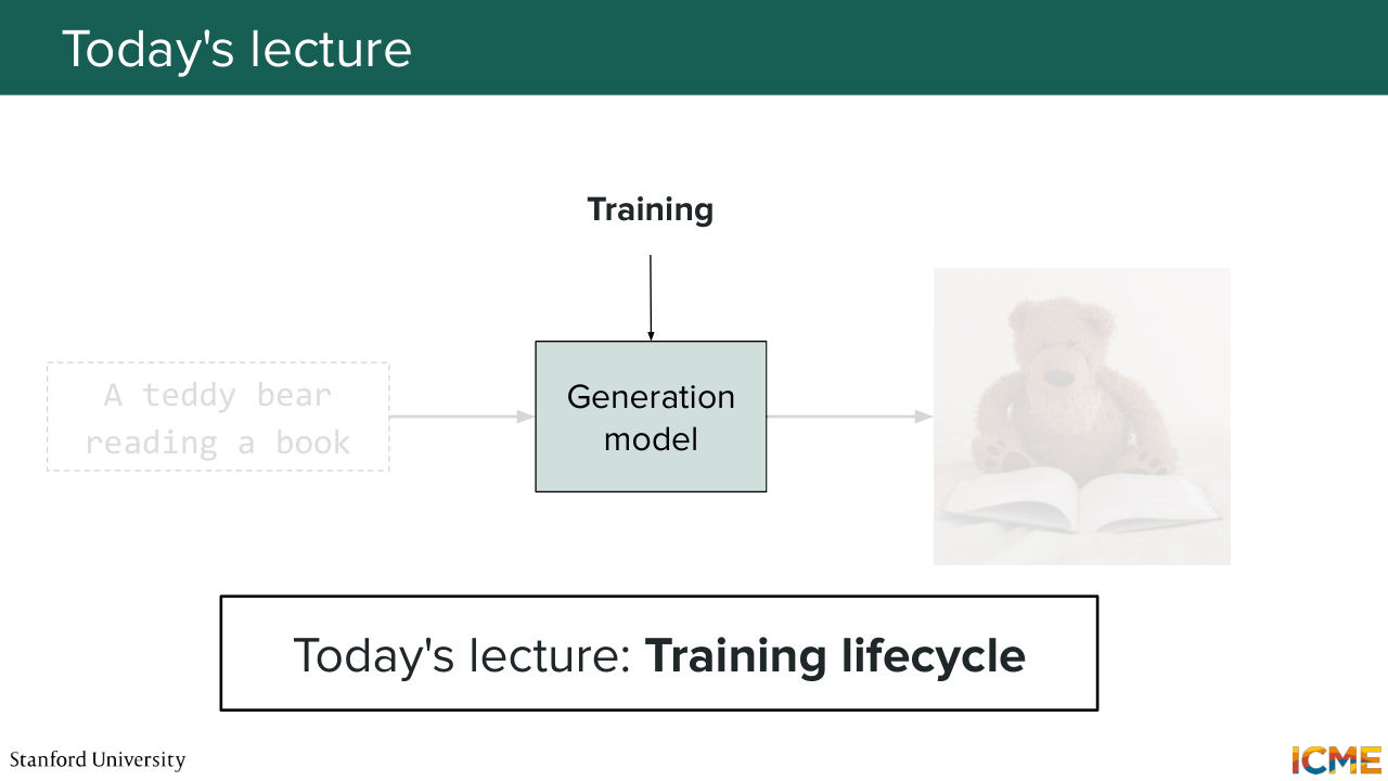
0:00 0:05 Hello, everyone, and welcome to Lecture 6 of CME 296. So today is a very exciting day because we'll be talking about how to train a model in practice,

0:20 a text-to-image generation model. And as you know, the first half of this class was all about preparing the foundational theoretical foundations for us to be able to do that. And in this second part, we'll be really talking about more the practical aspects, and today will be no exception. So as usual, before we start, we're going to just recap what we saw last time.
0:52 So if you remember last lecture, we saw the main image generation architectures.
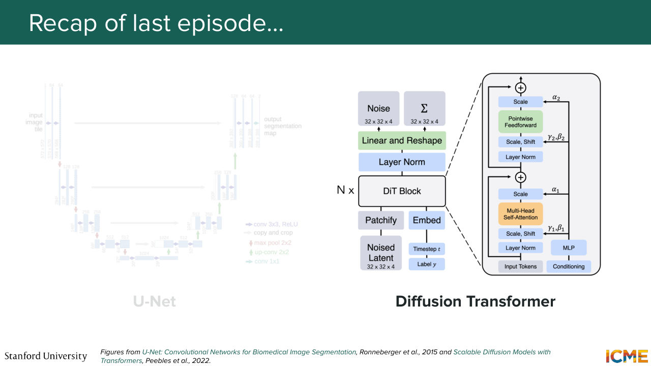
1:00 And we started with the big one, the UNet, which was trendy up until 2022. And we saw that among the things we wanted to see in an image generation model, we wanted the model that was able to understand the global structure of an image, also capture the local details, able to receive external signals, for instance, a condition, and be computationally tractable.
1:32 And we saw that the UNet was relying on an inductive bias.
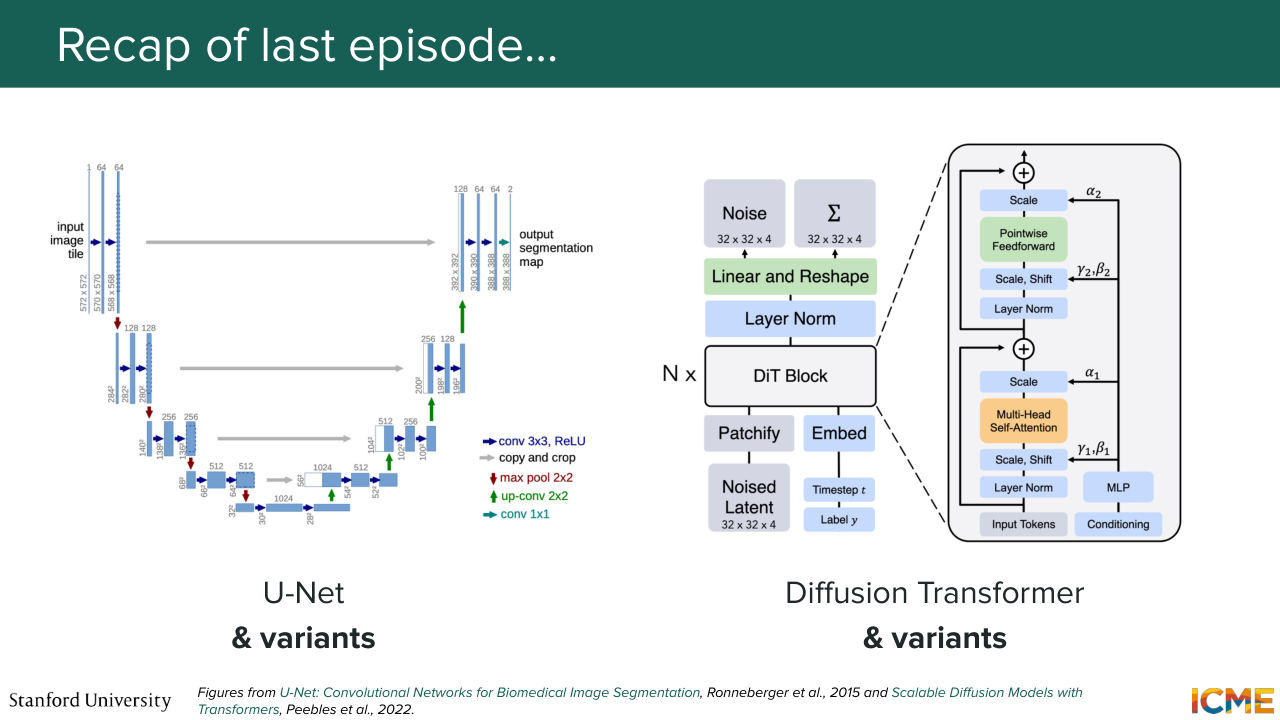
1:38 Which was something that was reflected by the convolution operation, which is mimicking how humans look at pictures.
1:49 And we saw that the unit was composed of two main phases. The first one is the downsampling phases, where we put an input, a noisy latent, that we then perform convolution operations and downsampling operations so that we can get a bigger receptive field that would enable us to have a global understanding of the input in the bottleneck.
2:18 So that was the first phase. And then the second phase with the upsampling phase, which was composed of upsampling operations, for instance, the transpose convolution, where we were able to get back to the dimension of interest, which is the same dimension as the input. And we saw that there are these copy-and-crop connections that
2:45 were allowing us to transport the local details that we were able to compute in the downsampling phase and couple that with the global understanding that we had, the global structure understanding that we had from the bottleneck. So that was the UNet. We saw that the UNet was great, but the UNet
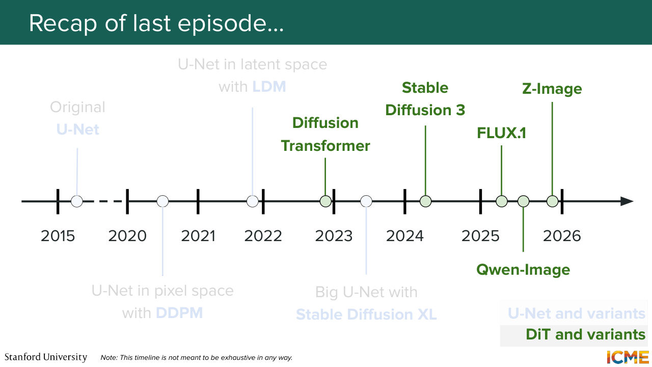
3:10 had a failure case, which was that there was no direct connection between different local parts of the image. And for an example, such as someone looking at oneself in the mirror. You need to be aware of the local details from two different parts of the image. So this was motivating us to look at another architecture, which is the diffusion transformer, which was published
3:42 in 2022, late 2022, which relies on the concept of self-attention, where each patch of the input latents attends to one another, allowing these direct connections to form. And as a result, we were able to have this concern mitigated. And we also saw a way to inject conditions into the architecture.
4:12 So we spend some time on the adaptive layer normalization, which was taking the condition and the time step as inputs that was modulating the token embeddings via this gates, shift, and scale factors. And we also saw that there were very many variants, actually. It was not just the diffusion transformer,
4:41 there were many variants of the diffusion transformer, such as the multi-modal diffusion transformer, which is now more trendy, which was looking at making the input text as a standalone modality that was being injected as input as opposed to an afterthought via the modulation, mainly because the adaptive layer norm was injecting
5:12 the condition across all patch embeddings in a uniform way.
5:18 And we didn't want to have that, so we also saw the MMD. And of course, these architectures are not the only ones that are out there. There are many variations. So hopefully, that lecture was a lecture that gave you the intuitive tools to at least understand why certain components are used. All good on this? So this was last lecture.
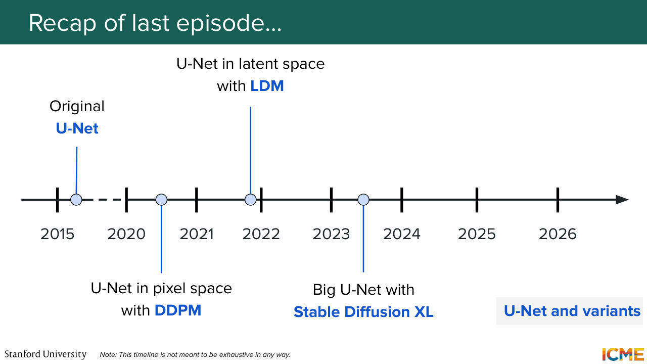
5:46 We also saw the timeline, which I briefly mentioned here. So UNet largely dominated the early 2020s,
5:55 if I can say it like this. And then the DIT-based models are dominating the architectures that are coming out nowadays, from end of 2022 onwards. And what are we going to do today? Today, we're going to focus on practical applications, on how we can actually train a text to image generation model.
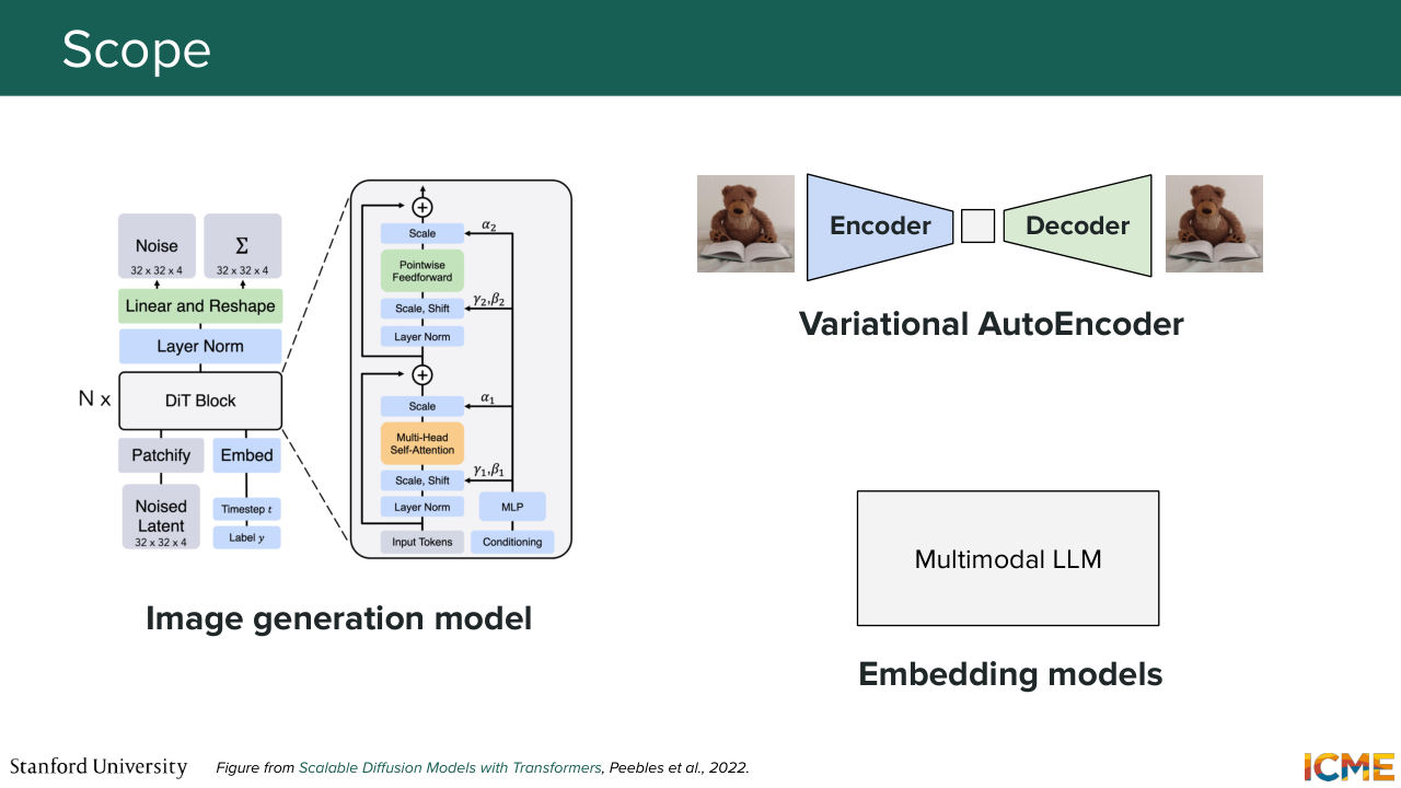
6:26 And I know so far we have seen different components of that overall system. We've seen the actual backbone that is allowing us to denoise the noise latents, which is for instance here a DIT-based model. We've seen that there is also another model involved, the VAE, which is allowing us to have a latent space in which we
6:55 can operate, which lowers the computational burden of our training process and generation process. And we've also seen that there are multiple models we could use that could embed conditions that we would then have as input. So to be clear, today we're going to focus on how to train the image generation model itself, and we're not going to focus on the VAE and the embedding
7:28 models. So just for reference, we will actually dig into embedding models next week with the multi-modal LLMs. But I'm going to just push it for next week. More on that soon.
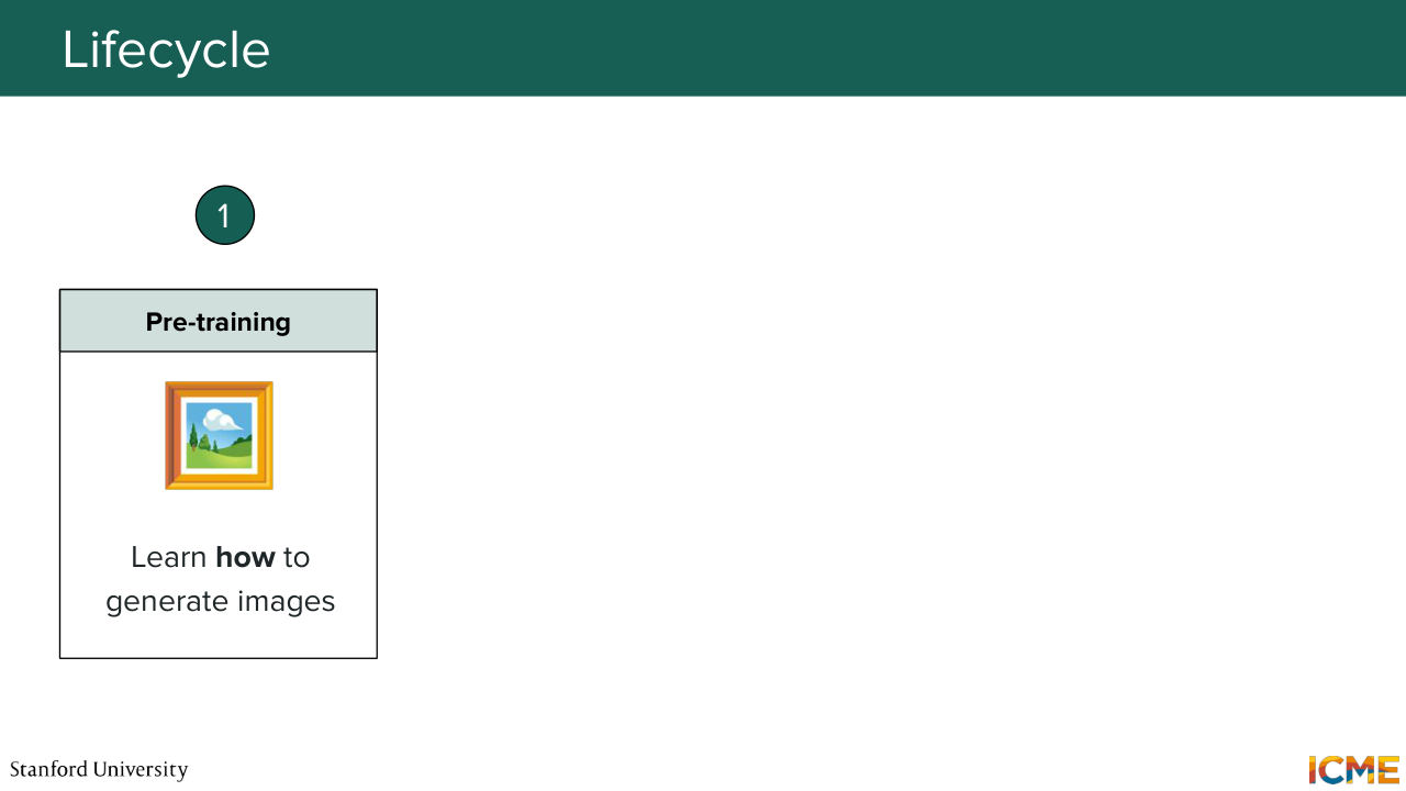
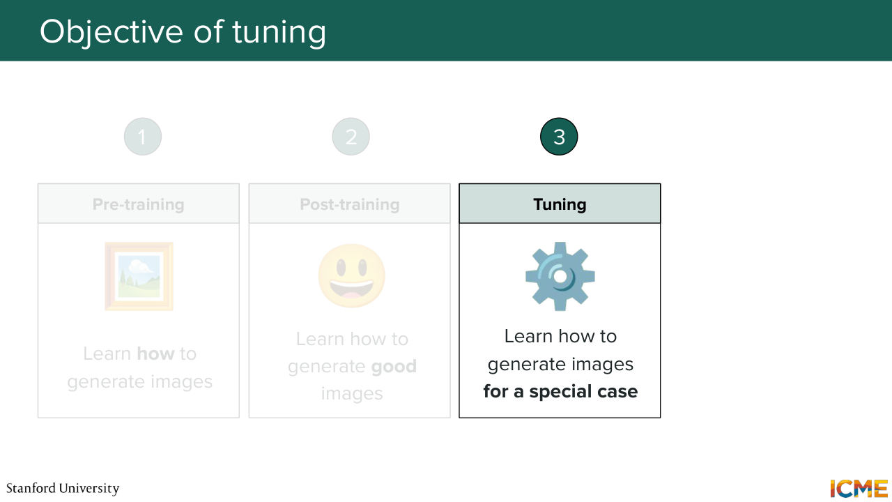
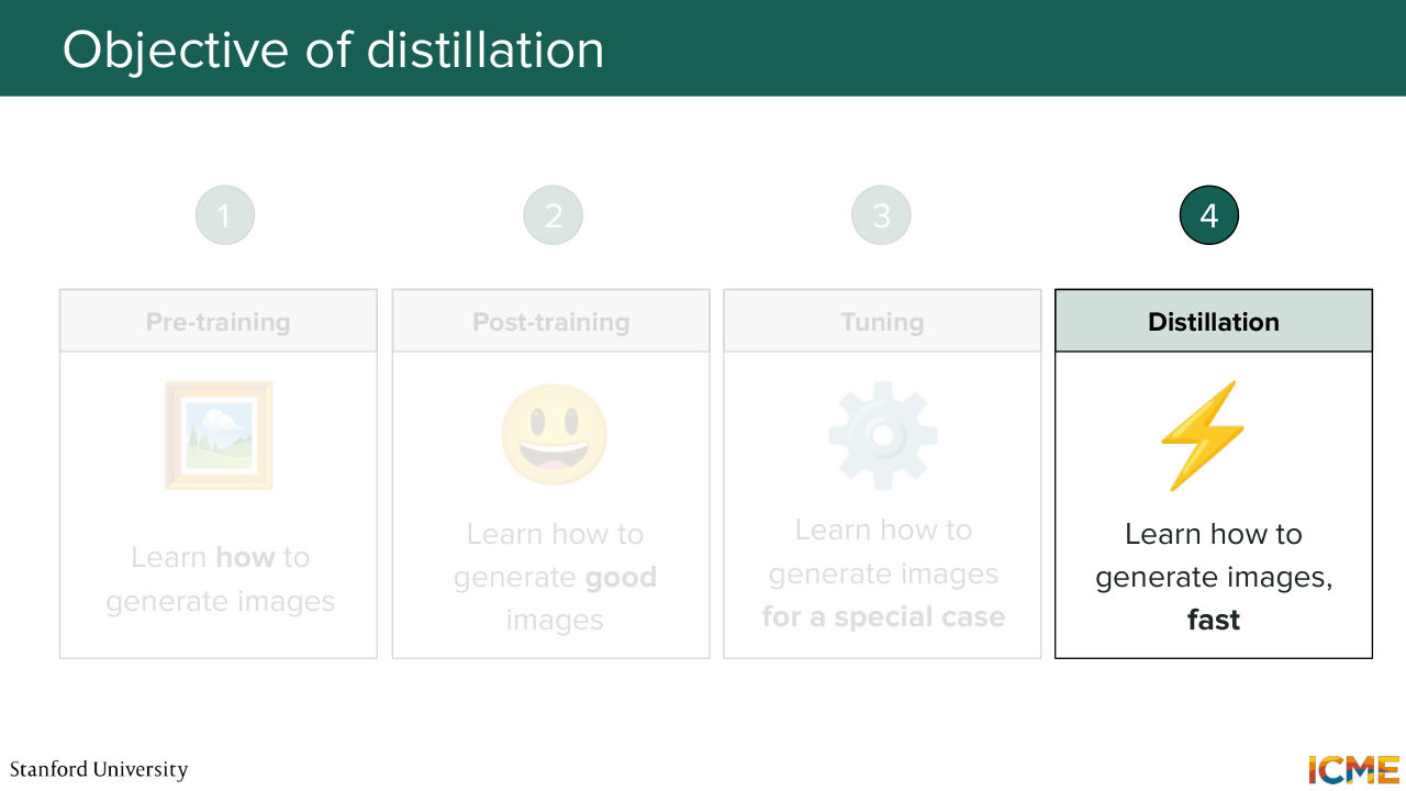
7:45 Cool. So let's start. And I just first want us to look at this whole problem at a very high level. And in particular, look at the overall process that allows us to go from an initialized model to a model that is able to work in production. So the first step, we have our image generation model.
8:16 We first teach it how to generate images, any images. This phase is typically called the pre-training phase. And it's quite compute intensive. It involves a lot of data and a lot of work on the data side. So that's number one, and it's a phase that all models go through.
8:43 Then we have a second stage that is called the post-training stage, where we take that pre-trained model that already
Shown briefly — discussed together with the adjacent slides.
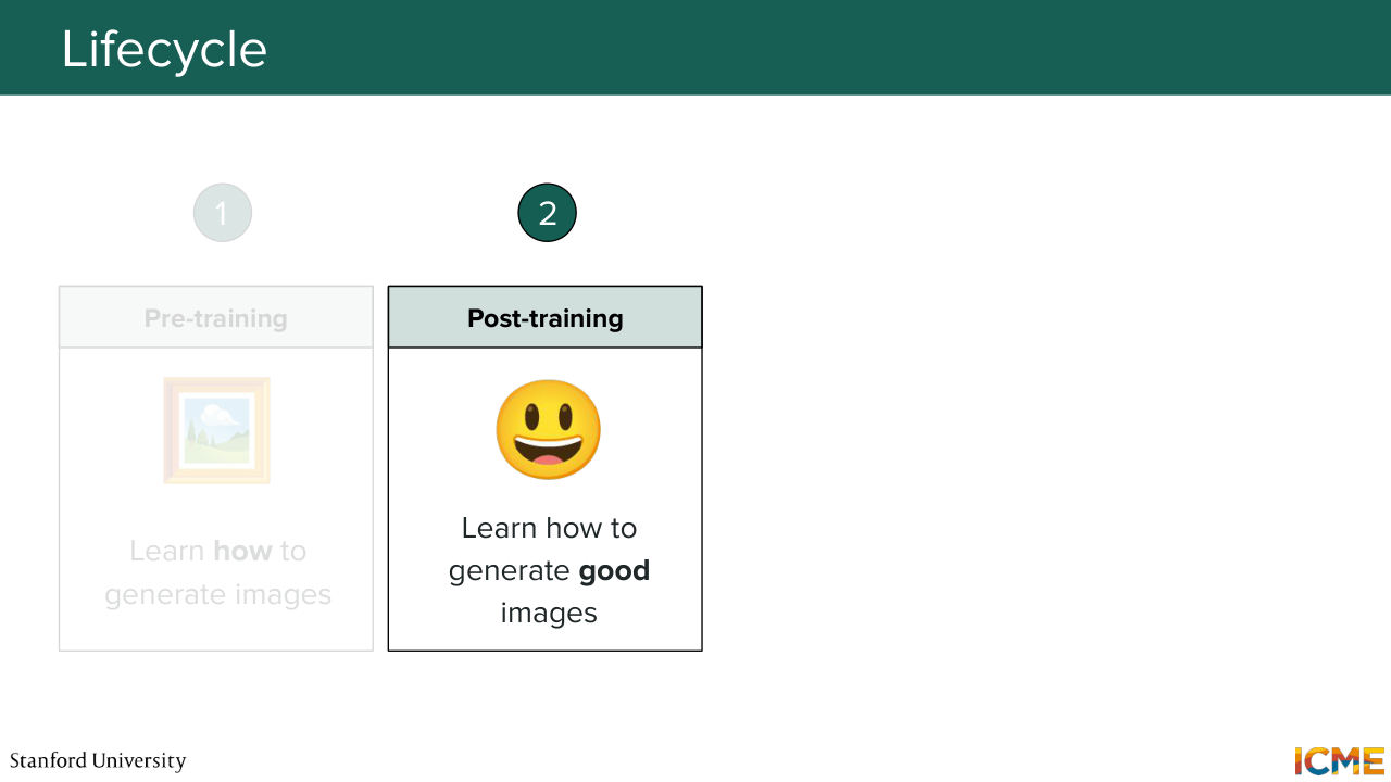
8:53 knows how to generate images, and we teach it how to generate
9:00 "good" images. And we will see what good means.
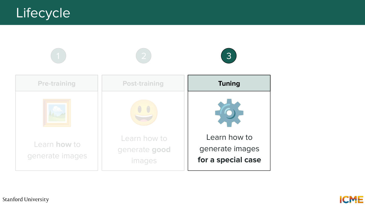
9:07 We could also optionally also personalize
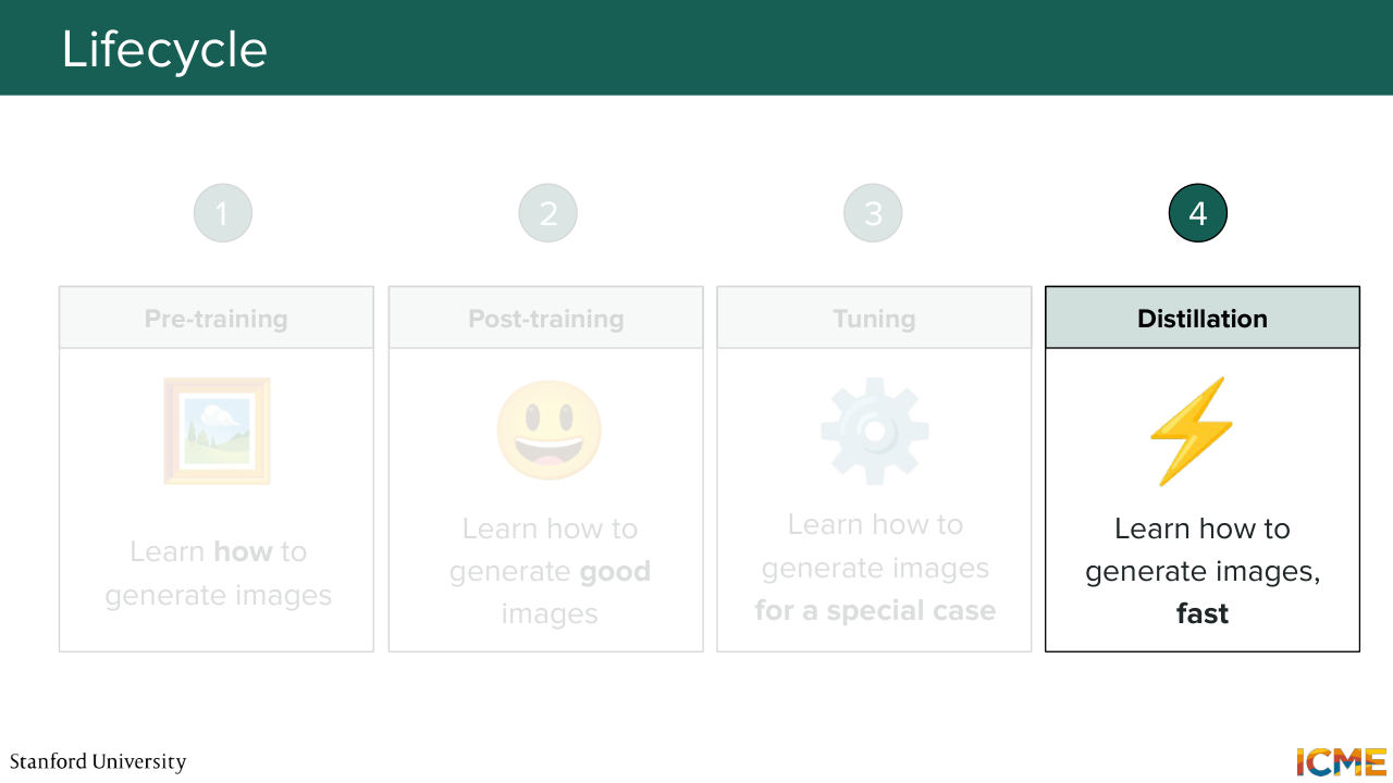
9:12 our model to generate specific kinds of images. And we will see this optional third step, which is here called tuning. And then at the end of this lecture, we'll also look at how we can actually make our model be able to work in production in an efficient way. And here we will look at distillation models
9:38 or distillation methods, I should say, that allow our model to generate samples in fewer steps, because we've seen that usually these image generation models, they're working in an iterative fashion. So you always have to have one the initial noise as input to get the let's say vector field, and then iterate on that many times potentially.
10:08 And here we want to shorten the amount of times we need to do that so that we can make this process just less costly and reduce the latency, which is typically what we care about for production use cases. Everyone good with the big, big steps? So we'll start with the first.
10:36 Even before starting, actually, we'll be talking about the loss that we will use for our training process.
10:44 And I think you already what the loss is because we've spent the first three lectures talking about three different perspectives on getting to that stage. So here, this part is mainly around just all agreeing on what those losses are and see what are the changes that happen in practice to these losses to make the training process more optimized.
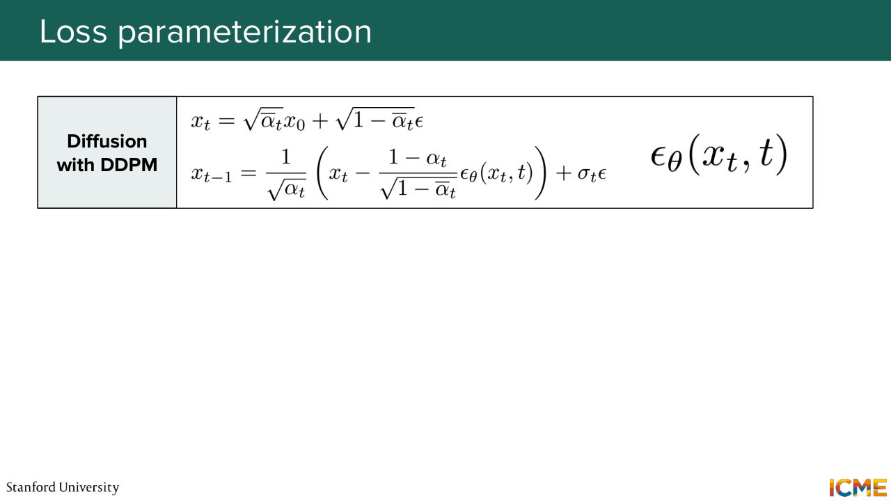
11:15 And you will see what I mean. So first, I'm going to recap what we saw during the three first lectures. So the first one, if you recall, was diffusion with DDPM where our thought process was we take clean images that we corrupt step by step, so you have this xt that
11:44 is a function of the clean image and the noise that you add. And we saw that we could derive a tractable loss, and you end up with a formula that is allowing you to denoise the noise with the formula on the slides by parameterizing a model that is geared towards predicting the noise to remove epsilon theta. And here, the loss is as follows. So it's the expectation of just the L2 distance
12:19 between your predicted noise to remove and the actual noise that was added,
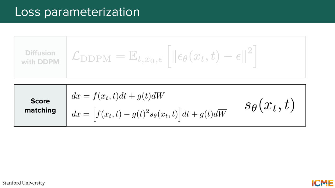
12:26 and it's an expectation over the time steps, the clean images that are part of your training sets, and then the noise that is typically sampled from a Gaussian distribution. Then in Lecture 2, we had this second perspective of looking at the same problem, which was, OK, in order to recover clean images, let's actually
12:54 look at where the clean images are by estimating the score, which is acting like a compass. And here we saw that there was a stochastic differential equation, way of putting this, which was given by dx is equal to some drift term and some diffusion term,
13:19 along with the continuous noise, which was the Wiener process. So this was the forward process. And then, the reverse process was something that was popping up the score. And this just highlighted the fact that we needed to estimate the score in order to denoise into clean images. And here, the last was an expectation over the score
13:53 that you wanted to estimate minus the actual score of the noise distribution.
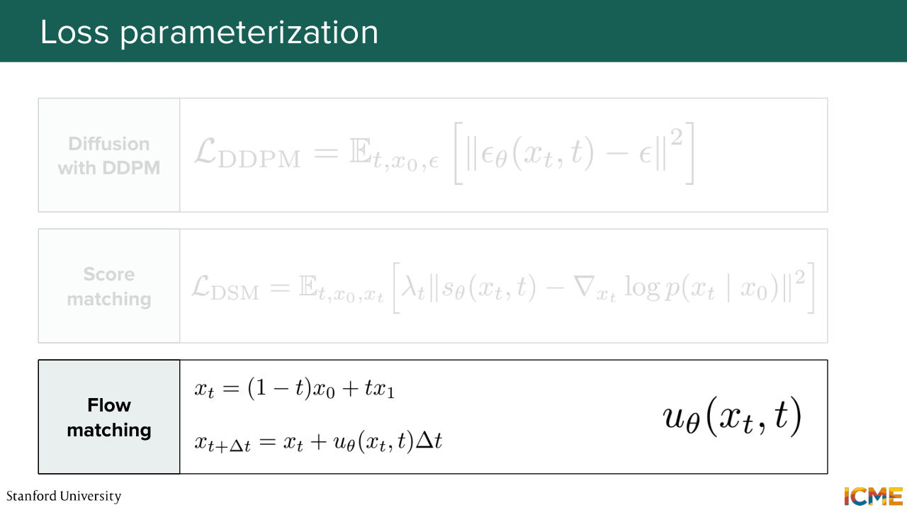
14:02 So that's the second loss that we saw. And then the third perspective, which was lecture 3, was the flow perspective, where we said that in order to go from noise to our target distribution, we're going to interpret that problem as a transport problem. And here, we focused on the velocity or also known as the vector field,
14:30 that could be used using an ODE solver like the Euler method. And we had a loss that was regressing the vector field by just taking two points. So one from the target distribution, x1, and then x0 from the noisy distribution, typically a Gaussian distribution.
14:57 And we ended up with this last function. Now, one thing I want to say, and maybe I've said it some time in the past, nowadays, people mainly focus on the flow-matching perspective. So I just want us to all be aligned that moving forward, by default, we'll be using the flow matching
15:25 loss as the default loss. Does that sound good? So let's look at this loss. So here what we're doing is we're optimizing on the parameter theta such that we minimize the loss on the slides in particular by taking the expectation over time steps over data points in the training data, so pdata,
16:00 and over noisy observations that are part of a Gaussian distribution. And in particular, we are taking-- so we were saying we were taking t drawn
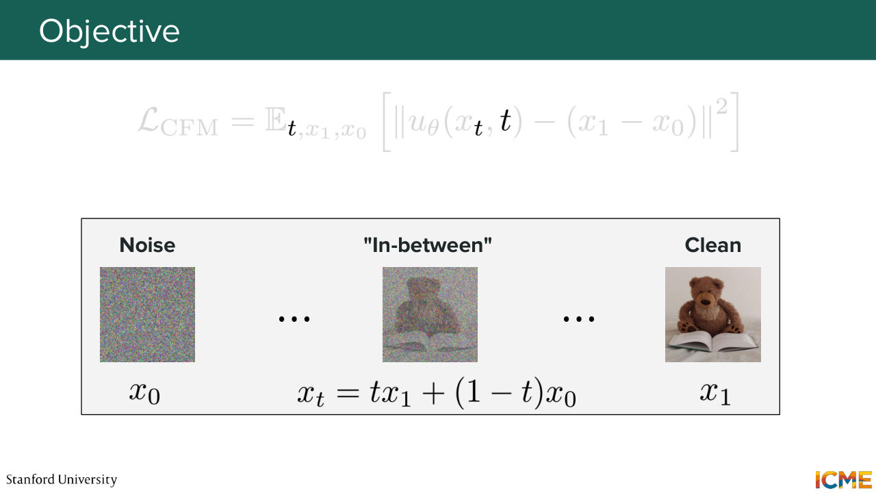
16:14 from a uniform distribution. And I just want us to pause on this statement and see if this actually makes sense. But first, just as a reminder, here by t we level where t equals 0 corresponds to a lot of noise, t equal to 1 means no noise at all, and t is somewhere in between means a little bit noisy.
16:51 So I'm going to ask you some questions. So let's suppose we want to figure out from an input that
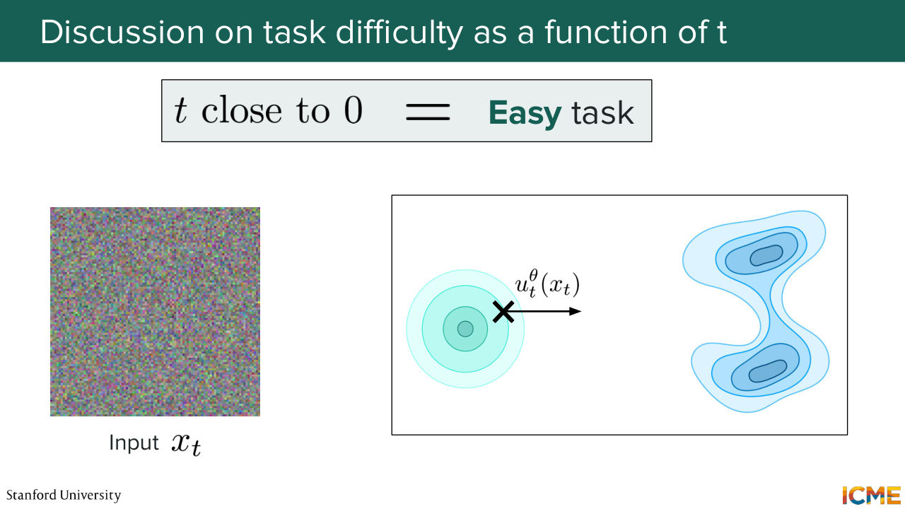
17:03 is extremely noisy, think of it as x0, whether making a prediction on where to go from x0 is an easy or a hard task. And so I'm just going to make our life easier. So if you remember the illustration we had-- so we have the noisy distribution that is the one on the left and then the target distribution on the right. So what we're saying is if we sample a noisy latent that
17:35 is very noisy, is the task of predicting where to go an easy task or a hard task? 17:49 Yeah, easy. Do you want to say easy? Yes, so it's indeed easy. Now, why is it easy? So at the very beginning, the input that you have is actually void of all information. You don't anything about where you're going.
18:10 So what your model will be incentivized to do will be to just try to predict if you want the average direction, where you need to go. So regardless of how much time you spend learning that, it will just learn roughly where to go, which will be if you want the mean of where all the observations in your target data distribution are.
18:37 So no matter how much time you spend in that region of noise, you will be incentivized to predict the mean of where all the observations are. So that's why I say it's an easy task. So now, how about if t is close to 1, meaning that we're already very, very advanced in the denoising process and there is almost no noise left? Is it an easy task or a hard task to where to go from there?
19:07 Hard? Yeah, OK, so we have one heart. Yep. Easy again. OK, so let's see. So let's try to think. So when t is close to 1, what that means is that the input xt is already almost clean.
19:36 So we're almost there. So what that means is you only need to make a few tweaks to little details to have a fully denoised image. And in that sense, it is actually an easy task because you already have an image that is almost clean and so on.
19:59 The illustration, it corresponds to if your observation is already part of the target data distribution, and you just need to do a small step towards having your final observation. OK, so let's do the last one. How about if your input image is not super, super, super noisy,
20:24 it's not almost clean, it's somewhere in the middle? Is the task easy? Is the task of knowing where to go easy or hard?
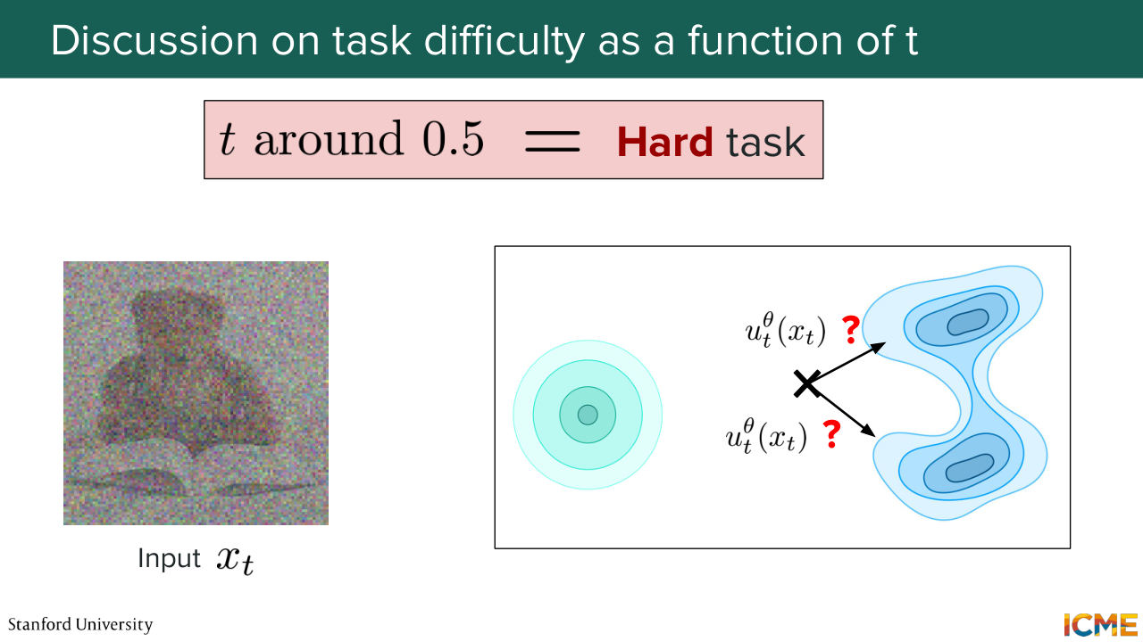
20:38 Yep. Hard? And same here? OK, so yeah, you're completely right.
20:45 And to illustrate the point that you're saying, we are indeed in this space at a point
20:53 where we need to figure out about where to go. But even thinking about it from an intuitive perspective, let's assume that your target distribution is composed of images of teddy bears. If you're in the middle, then it means that roughly what the body is like, what the head is like, you know a little bit where the arms like, but there's a lot of things that you need to figure out about where to place. You need to figure out what kind of texture
21:23 you want your teddy bear to develop. You need to put the eyes. You need to put a bunch of things. And these are all hard decisions that you need to take at time steps that are typically in the middle. And for that reason, t equal to 0.5 is a hard, hard task for the model. So if you remember, what we saw was
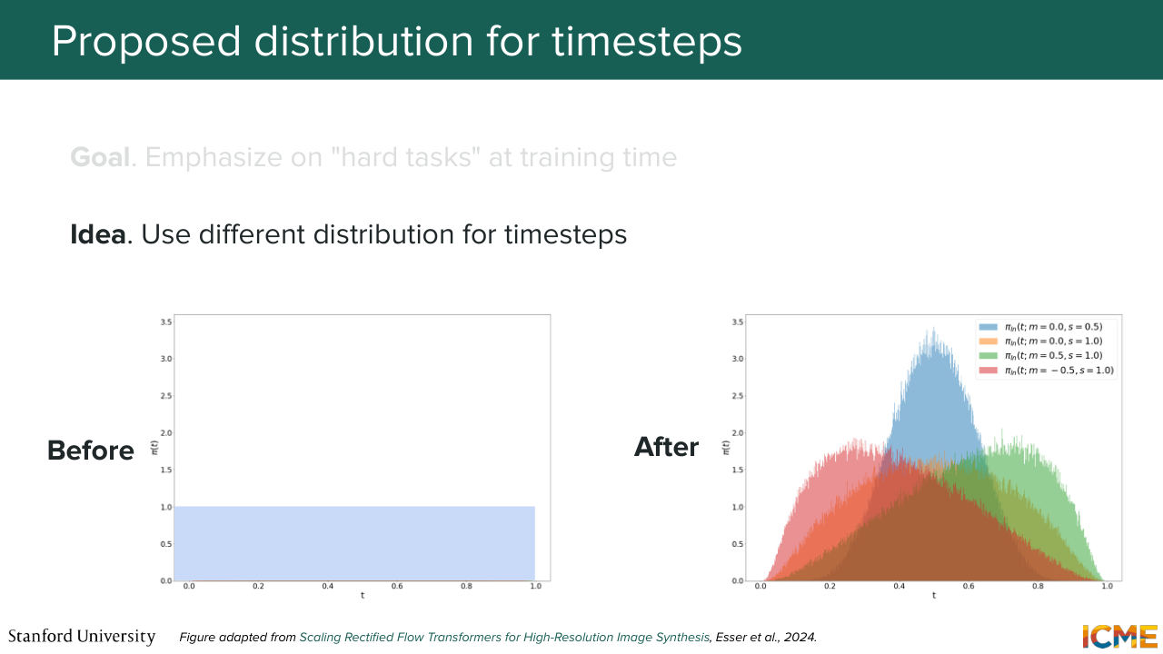
21:52 that we were drawing our time step when computing the loss from a uniform distribution. So what that means is we're asking our model to try to be good at predicting the target as many times for easy tasks as much as for hard tasks.
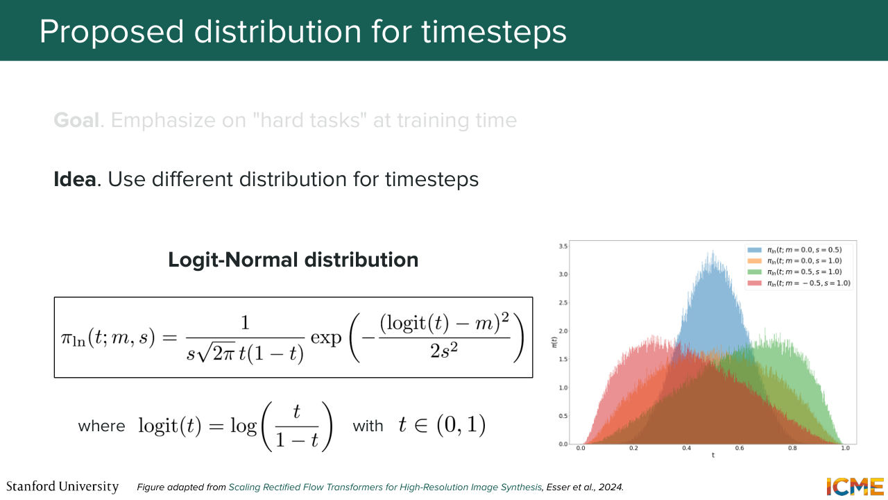
22:16 And this is the reason why, in practice, people actually do not sample the time step from a uniform distribution.
22:27 They actually sample from another distribution, which we're going to see in a second, that emphasizes on middle steps more than it emphasizes on either the early or the late, late steps. And the distribution that people in general use typically is called the logit-normal distribution. So the formula on the slide may look scary, but it's actually quite simple.
22:58 So what we're saying is-- so first of all, I'm going to define what logit means. So the logit of a quantity-- so let's suppose the logit of our time step t. --is defined as the log of t over 1 minus t as follows. And so t is between 0 and 1. So if t is between 0 and 1, then logit of t
23:31 is anywhere between minus infinity to plus infinity. And what we're saying is if we sample x from a normal distribution, which is between minus infinity to plus infinity, then if we express t as a function of x,
24:03 which-- I'm looking at the time, we will probably not do. You will have something like this, which is just a sigmoid. And that quantity will have a distribution that will be really centered in the middle. So you may ask me, "Well, why do you not sample directly t from
24:32 a normal distribution?" Maybe it's a question you ask. But the reason why you don't do that is the normal distribution is a distribution that can take any values, and you only want values between 0 and 1. So that mathematical trick is just a way for you to guarantee that in between 0 and 1 because here the sigmoid is between 0 and 1.
25:03 Does that make sense? OK, great. I just want this formula or this distribution to not seem like it's coming out of nowhere. So the good thing with this distribution is you can tweak the way the distribution is shaped. So you can play with the mean and the standard deviation, so you can shift it towards the time steps that you care about.
25:31 So for instance, if you in your use case care about the later steps, you can do that. And so that is the reason why people use that distribution. But I'm not done with time steps.
25:47 There's another thing I want to talk to you about. So we're talking about noise levels,
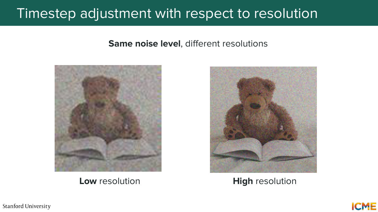
25:54 but what we actually care about is how much noise is perceived by yourself. So if you take the same image, one in low resolution and the other one in high resolution-- and if you apply the same amount of noise, which, from the slide, I hope you can see, that the one on the left, the low resolution one, feels more noisy than the one on the right.
26:27 So same image, different resolution, but same noise level. The one on the left feels more noisy than the one on the right. So something tells you that you also need to take that into account in some way. So right now, we're not taking that into account, but not for long. So you will see that in papers, there is this concept of time step shifting
26:55 as a function of resolution, where the idea is to rescale the noise level in a way that reflects the perceived noise that you see. And so I just want to pause on this concept for a second. Why would you perceive a low-resolution image would
27:20 be more noisy than a high-resolution one for the same noise level? Why would you have to do that? Or why would you think that? Well, there is one thing with images, which is that they have a lot of spatial correlation. Meaning for a given pixel, you have-- you are very likely to have pixels around it that have
27:44 the same value or same color. And so remember that when you add your noise, you're adding Gaussian noise with mean 0. So what that means is if you have very few pixels, when you're in low resolution, then if the pixel that is responsible for, let's say, the color that characterizes how good your image looks, let's say, at a particular angle--
28:15 if that one gets noised, then you're losing that information. You're not able to see it anymore. But in the high-resolution case, you have multiple pixels surrounding that region. So even if one gets noise, the other one gets noise the other way because remember that the mean should be equal to 0, the mean of the noise, added noise, should be equal to 0, you will still
28:41 have an average value that will reflect the underlying pixels much more compared to the low-resolution case. So for that reason, I hope the statement that I'm making, which is, for a given noise level, things feel more noisy for low-resolution images compared to high-resolution ones--
29:07 I hope that one is intuitive. I'm going to pause for a second. Does everyone agree with my statement?
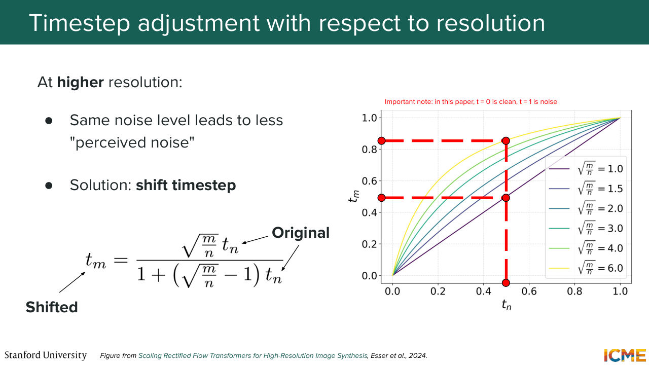
29:14 Yep? OK, so there is, again, a very scary formula on the slides. The reason why there is just to show you how people shift time steps in practice. So I would first want us to look at the chart on the right. So you see tn and tm. So here, let's assume you have two images, one of resolution n
29:46 and the other one of resolution m, where n is smaller than m. So here for a given tn, you would want to have a higher tm because for a low-resolution image, for a given noise level, you would want that noise level to be higher for the high-resolution image,
30:16 for the perceived noise to be the same. So that is what this formula is saying. But I know it's not intuitive, so what we'll do is we'll take 10 minutes to try to understand what that is about. So the formula on the slide is all about
30:45 reflecting the change in uncertainty of pixel values that are noised under different resolutions. So let's assume that we have an image, so you can think of it as this, with-- OK, I'm being quick. So you have, let's say, height and some width.
31:14 And let's say that n-- so let's say m is this one. And let's say you have a smaller image with, let's say, h, little h, and little w, and n is equal to h times w. I'm just saying that n is a lower resolution than m.
31:42 That's just what I want to say. So here, what we want to do is to try to quantify the uncertainty of what the underlying pixel values are in the case where we have noise for both cases. So what I propose to do is to just assume that these images-- let's assume that they all have a certain value as pixels. So pixels have three channels.
32:16 Let's assume here that we have only one channel, one value by component. So here, let's assume that each of these is, let's say, equal to some value c that is constant. So far so good? So let's assume that for a given let's
32:41 say index i that tells you about where you are in the image, and for a given noise level t, the value at that index is something that is given as a function of C, the value of your pixel, and the amount of noise that you're adding to it. So here I just need to put the noise level.
33:19 So I told you in lecture one that people use different conventions for time steps. And it just happens that the formula here and the paper here, they used the reverse convention when it comes to time steps. And in particular, they used t equals 0, means clean, and t equals 1, means noise, which is the opposite
33:49 of what usually people do. But in order for us to be consistent and end up at the same formula, we will just assume that is the convention that we're going to use. So here, what we're going to say is it's 1 minus tc plus t epsilon. Does everyone agree with me? So this is the value of the noise pixel at the noise level
34:20 t. So here epsilon is drawn from a normal distribution. And so what can we say about this one? So we assume that this quantity is a constant, but we don't what that quantity is when we look at an image. So our goal here is to quantify the uncertainty
34:52 if we were to estimate c, which is a constant. So what I'm going to do is to try to quantify the uncertainty of c. So here, just because we have n elements, so m here and n here n elements, I'm just going to leverage the fact that we have this n elements to take the average over all pixel values.
35:24 So I'm going to sum over, let's say, i my index, that's between 1 and the number of pixels, of the zi(t). And I'm going to call this zt bar for average. So here, this thing is a constant, so it doesn't move. And this thing just gets-- so here, I'm going to write this here plus the average.
35:59 So I'm going to put the t here. The sum of y from-- sorry, sorry. The sum of I from 1 to n of the epsilons, which are-- as a function of i. Because the noise here is different from one pixel to another. So here what I wrote is that the average value of a pixel
36:26 is 1 minus t times c plus t over n of the sum of the noise values. So you're going to see why I did that. 36:51 So here, I just want to remember our-- to remind you of our objective. Our objective is to quantify the uncertainty in estimating c.
37:05 So I want us to first see that zt bar is equal to a constant plus a sum of independent Gaussian variables. So what you can see about-- what you can say about this quantity is that its mean is 1 minus t times c. And its variance-- let's see.
37:38 So t over n is a constant. So the variance of a constant is just the constant squared. And then the variance of each epsilon i is 1, and you're adding n of them. So it's n times 1, which is t squared over n. OK, great. So why am I doing all of this? I just want to remind all of us that what we know-- what we want
38:17 is to estimate the uncertainty of C. So what is a good estimator for C? So C-- here, we see that zt bar is equal to minus C times C plus something where the mean is 0. So a good estimate of C could be 1 over 1 minus t times zt bar. And what we want to quantify is the uncertainty in estimating c.
38:52 So what is the uncertainty around estimating c. So this thing is a constant. So the variance of a constant is just-- so sorry, the variance of a factor in front of something else is the constant squared times the variance of this one, which is t squared over n.
39:21 So what we're saying is that the standard deviation of our estimate is equal to the square root of the variance, which is t over 1 minus t times 1 over square root of n. OK, so what does that mean? That means that the uncertainty that we have around
39:53 determining what the pixel value, underlying pixel value, is a function of 1 over the square root of the resolution. So as we increase the resolution n, that uncertainty gets smaller. And so in order to get that derivation, which I don't think I will do, it is just some math, you would just equal that uncertainty for n.
40:30 So it's t under subscript n here. And you do the same for m. So you get exactly-- so the noise level at time step-- for resolution m will be as follows. And the goal that we have is to determine the time
41:00 step for resolution m such that the uncertainty of determining the pixel value is the same. So you just need to take these two quantities and just say that they need to be equal, and you find tm as a function of tn. Does that make sense?
41:33 So the low-level derivation is not that important. What is important is just the mindset, which is that here we want to shift the time step for higher resolution, such that we match this perceived noise that we have.
41:57 And so hopefully, when you take a look at that formula, you're not thinking, "OK, where does that come from?" OK, cool. So I think we're done with the time steps. Any questions on this? Yep. What is c again? Yes. So the question is, What is c again? So this was actually a toy example
42:23 that we had where we said let's assume that we have an image where all the pixel values are constants, all equal to c. So c is the value of the pixel that is across all our image in this toy example. And the only problem with c-- we know it's constant, but we don't what c is because we have noised that image.
42:50 And this whole derivation is about quantifying our uncertainty of what c is if we were to estimate it. And what we said was that we could quantify the uncertainty through this standard deviation. And what we said was, depending on the resolution
43:14 at which you're operating, that uncertainty is higher or lower. And in particular, that uncertainty is lower as the resolution gets higher. And this is all because you can actually perform your estimation by averaging across all pixel values, which are getting bigger and bigger when the resolution increases. Does that make sense? OK, perfect. Yeah, yep. So the question is, we said that the diffusion process is taking
43:44 place in the latent space, so m and n are in the latent space? Yes. Yep. OK, perfect. Let's move on. We're done with the time steps.
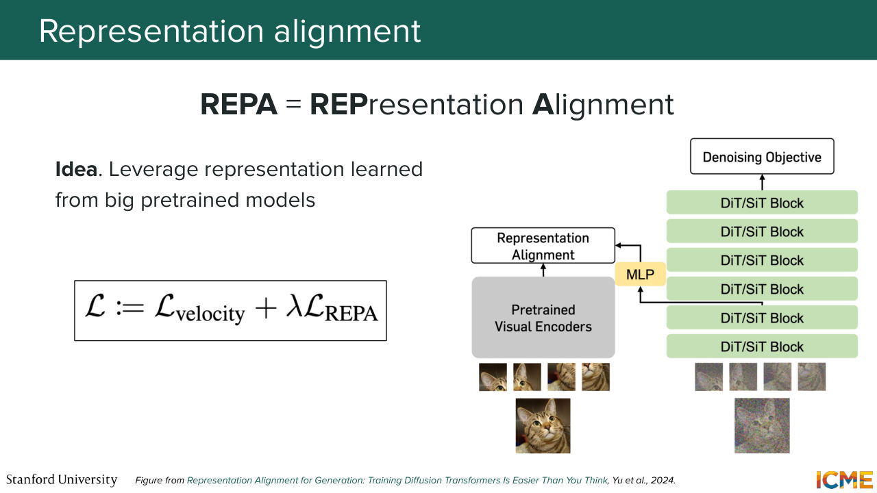
43:58 Now we're going to the next training trick that I wanted to talk about, which is helping our model with learning representations faster. And how do we want to do that? So here, the whole idea is to leverage the representation that some already pre-trained encoders have learned
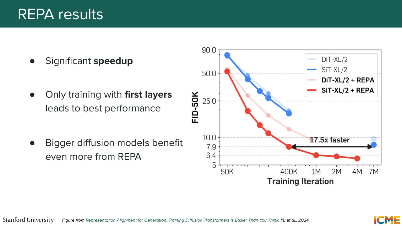
44:27 and incorporate that, and incentivize our model to match that representation. So in other words, it's as if you want to learn about a topic, and I come and get you a book about that topic. So you can learn faster about the topic, so it's exactly the same mindset. So here, REPA is the name of the method.
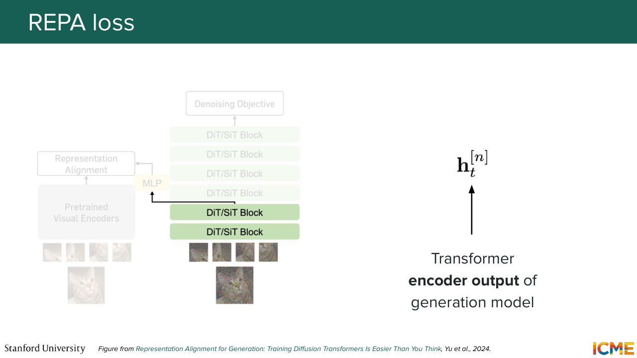
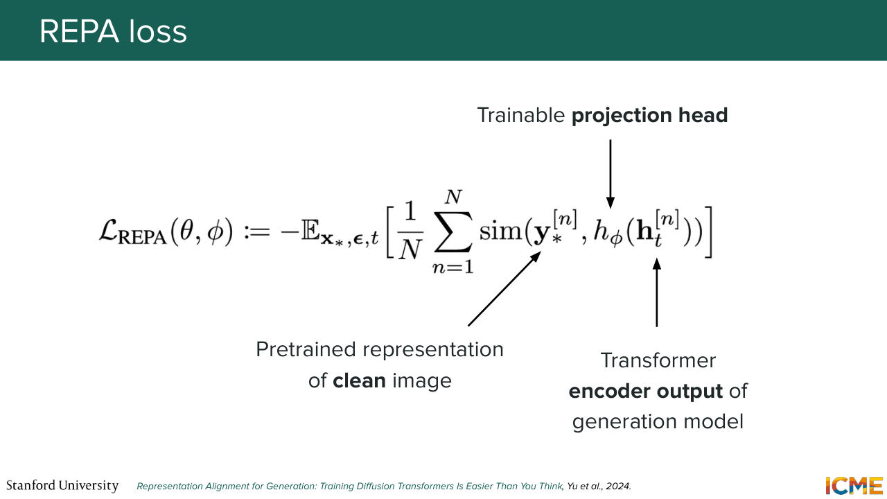
44:53 It stands for Representation Alignment. And it consists of coupling your loss with a loss that reflects how similar the representations that you're obtaining within your diffusion transformer is with respect to what the pre-trained encoder is giving you. So that's what REPA is about. So let's go step by step. Here, we mentioned the L loss for REPA,
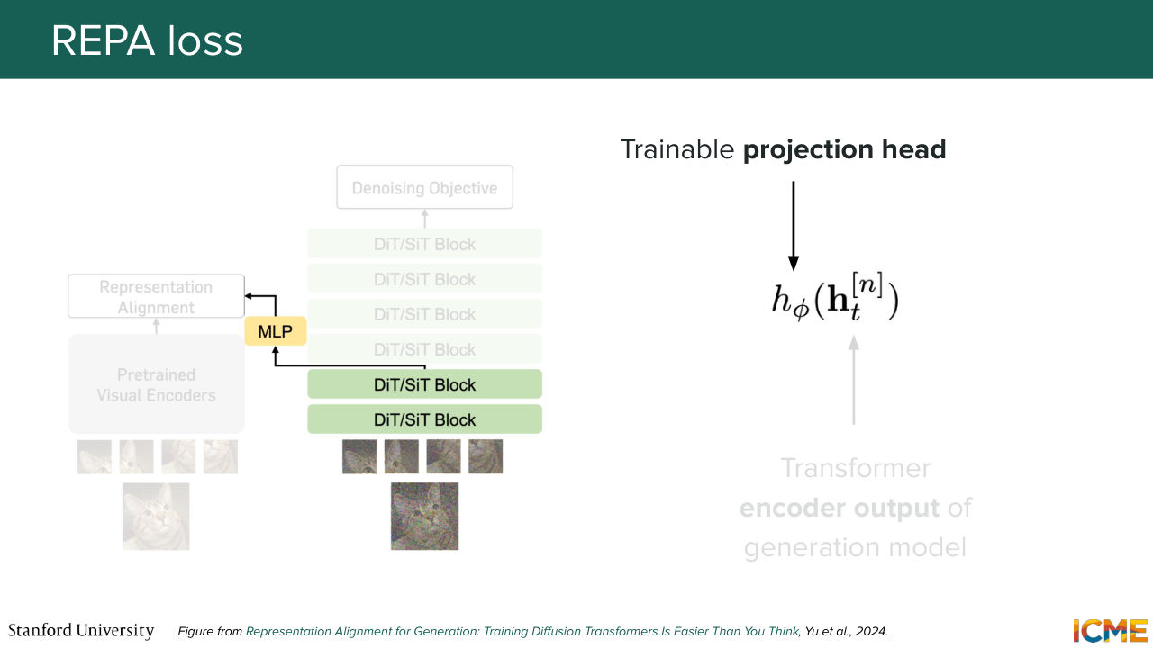
45:26 but we have not seen what that loss is. So we're going to see now. So here what we're saying is in the diffusion transformer, you have several layers. So what you're saying is you're taking the encoded output of a given layer. So let's call that ht. And here n, I believe, represents the patch, let's say, for a given patch n. And let's project that on a space where
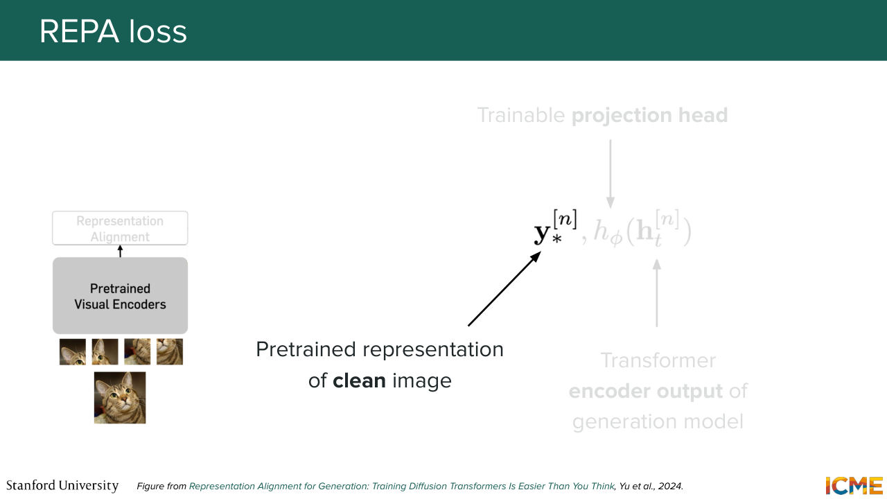
46:00 we can compare the equivalent clean patch representation from the pretrained encoder, and then have a similarity operation between the two. So in other words, we will be penalizing our model for having a projection of the encoded output of a given patch.
46:25 That is, noise we will penalize our model from this being dissimilar from the representation given by the pre-trained encoder of that same patch, but cleaned. So why do we do that? So as I mentioned, we're giving a book to someone who's learning about a topic so that they can learn faster. And that's exactly what happens.
46:54 So what we're seeing with this strategy is that it speeds up training significantly, so here on the order of 18 times. So this graph represents some measure of how good your images are as a function of the training iteration. And what the authors did was just try out a bunch of different--
47:19 they tried a bunch of things. So they tried different models. They tried different layers. They tried-- so they did a lot of ablation studies. One of the things that they saw was if you were to perform that loss on the embedding from earlier layers, then you actually get better results. And I just want to pause on that statement for a bit
47:47 just to understand why that is the case. So our diffusion transformer gets to compute a prediction of where it wants to go. And in that sense, the later layers may actually involve more local details rather than a semantic representation of where you want to go.
48:19 And so here that pre-trained encoders, some of them, what they're good at is representing things in a semantically meaningful way. And so one can understand these facts by saying that, OK, we actually want the representation from a layer that is supposed to output something that is semantically meaningful to align
48:44 with a semantic or semantically meaningful representation. I just wanted to vocalize a possible interpretation. And then the last thing I will say is that an interesting thing is that the bigger your model, the faster or the more benefits you have from this method.
49:07 Cool. And the REPA was published in 2024, but it is a technique that I have personally seen in a lot of new papers, so worth keeping in mind.
Shown briefly — discussed together with the adjacent slides.
Shown briefly — discussed together with the adjacent slides.
Shown briefly — discussed together with the adjacent slides.
Shown briefly — discussed together with the adjacent slides.
Shown briefly — discussed together with the adjacent slides.
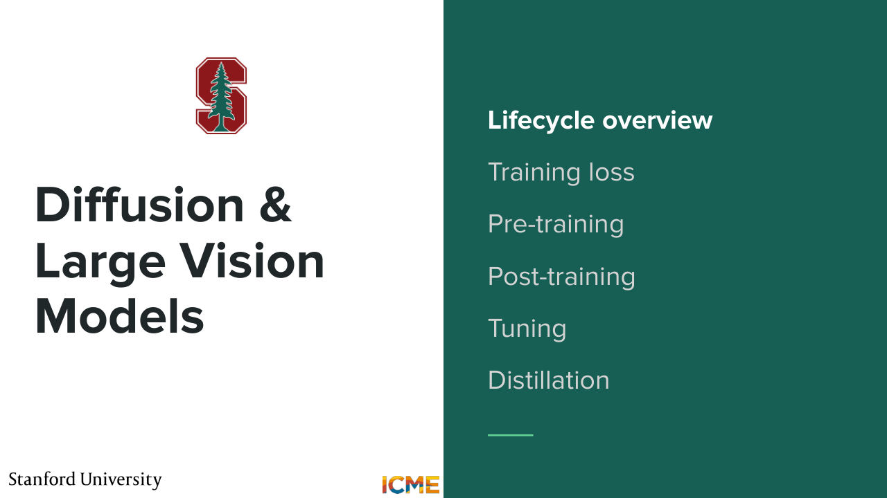
49:20 And that is concluding the first preliminary parts.
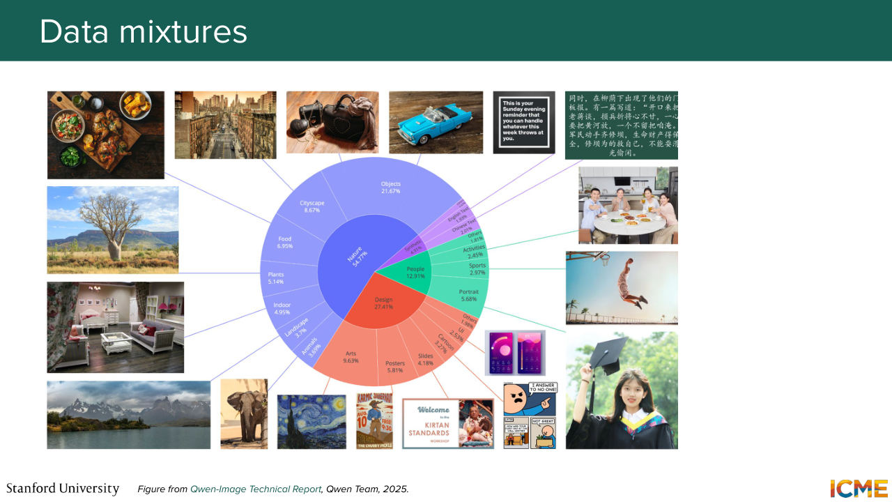
49:26 So now we're going to first start the first step of the lifecycle, training lifecycle, which is pre-training. And so as a reminder, in this first step, the goal is to teach our model how to generate just images. And so here there is a lot of work that goes into what kind of images
49:53 you want your model to learn from. And so I just have this one slide, which is coming from-- so it's an image from the Quinn technical report, which just tells you that this is a very time-consuming work that's involves data pipeline with a bunch of filtering, different resolutions, cleaning, and so on. So I just have one slide to illustrate this,
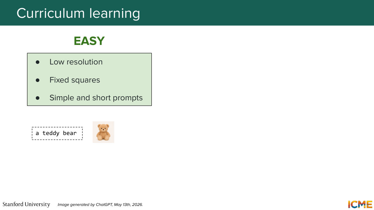
50:19 but it's a very time consuming step. So just know that this is an important part of the process. There is a concept that I want to talk to you about, which is called curriculum learning, which is about teaching your model on things in a progressive manner on the scale of difficulty. So in other words, here, what we want
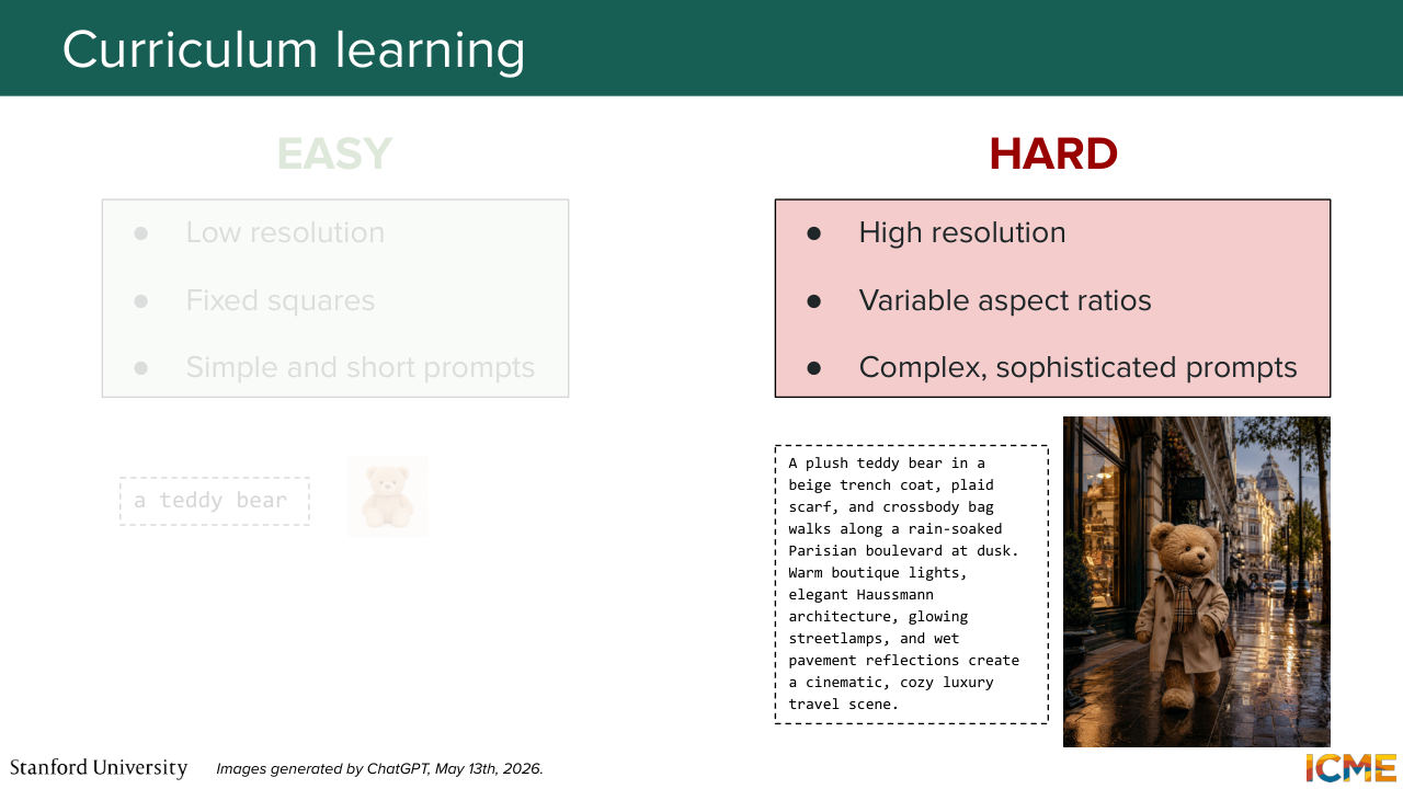
50:48 is to teach first our model on doing the easy things before doing the hard things. And this is a practice that is typically something that people do as this just helps the model learn better. And so here, by "easy" I mean low-resolution images that are of very easy aspect ratio, so fixed square. You can think of that. And then the input text is simple and short,
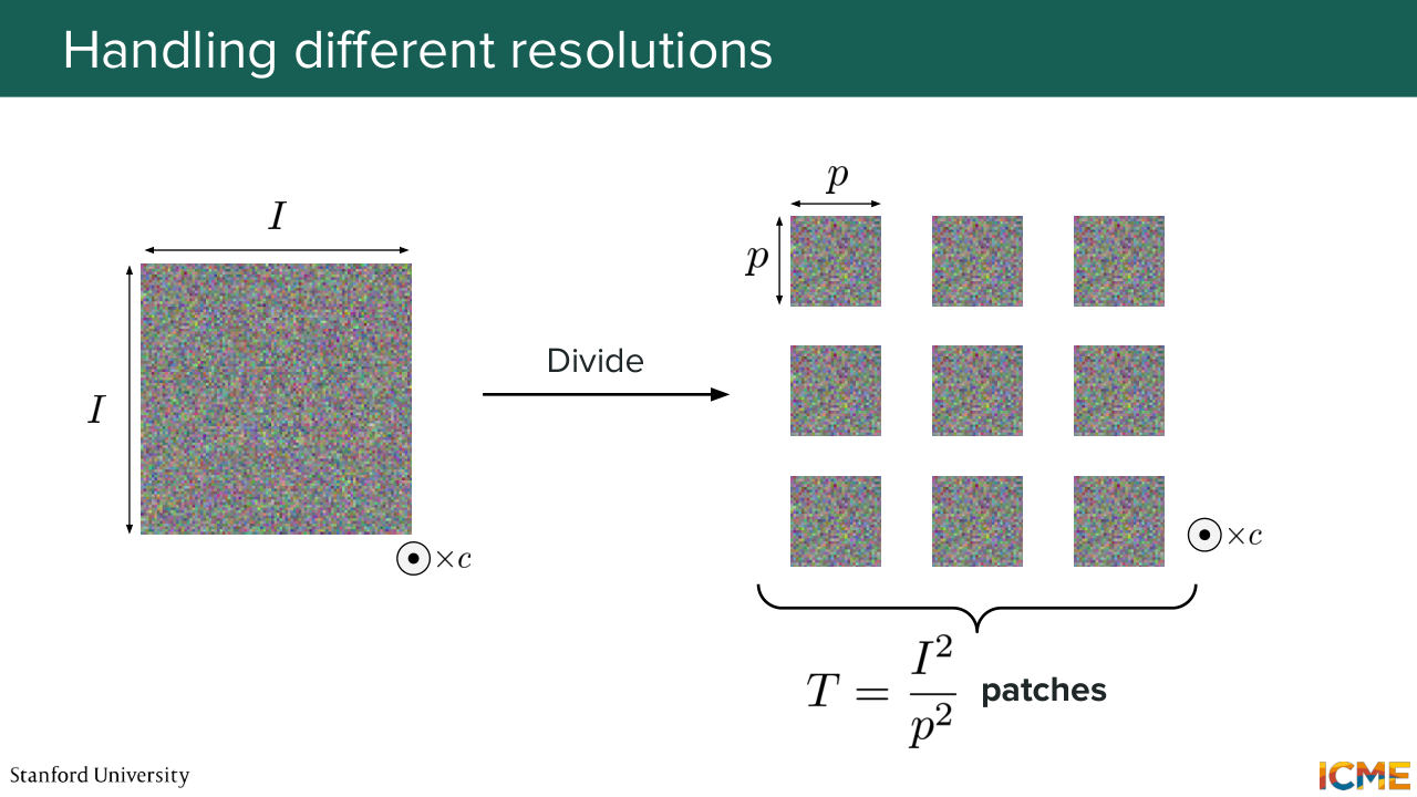
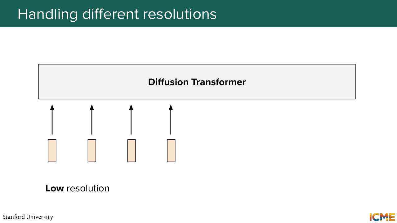
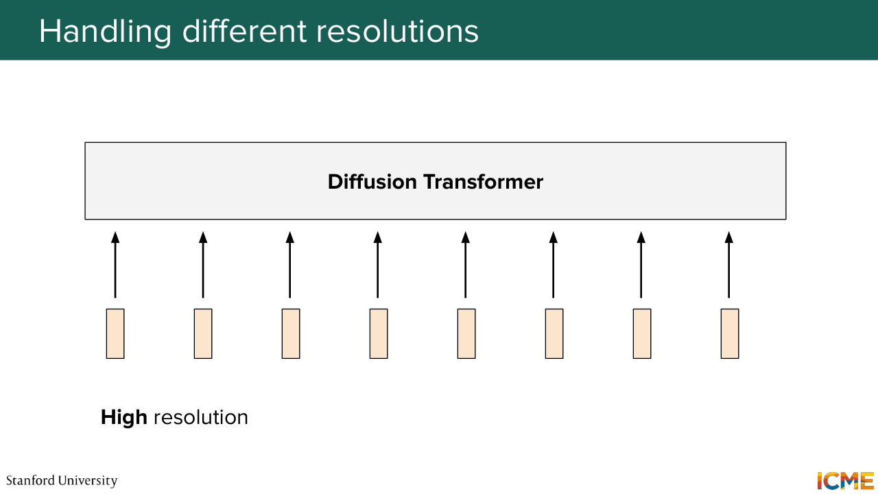
51:18 so for instance, a teddy bear. And then the hard part is if you want to predict something that is of high resolution, different aspect ratios. It's not a square anymore. And then, your prompt can be much, much more complicated, such as the one on the slides. And now you may ask me, well, how would you handle images of different resolutions?
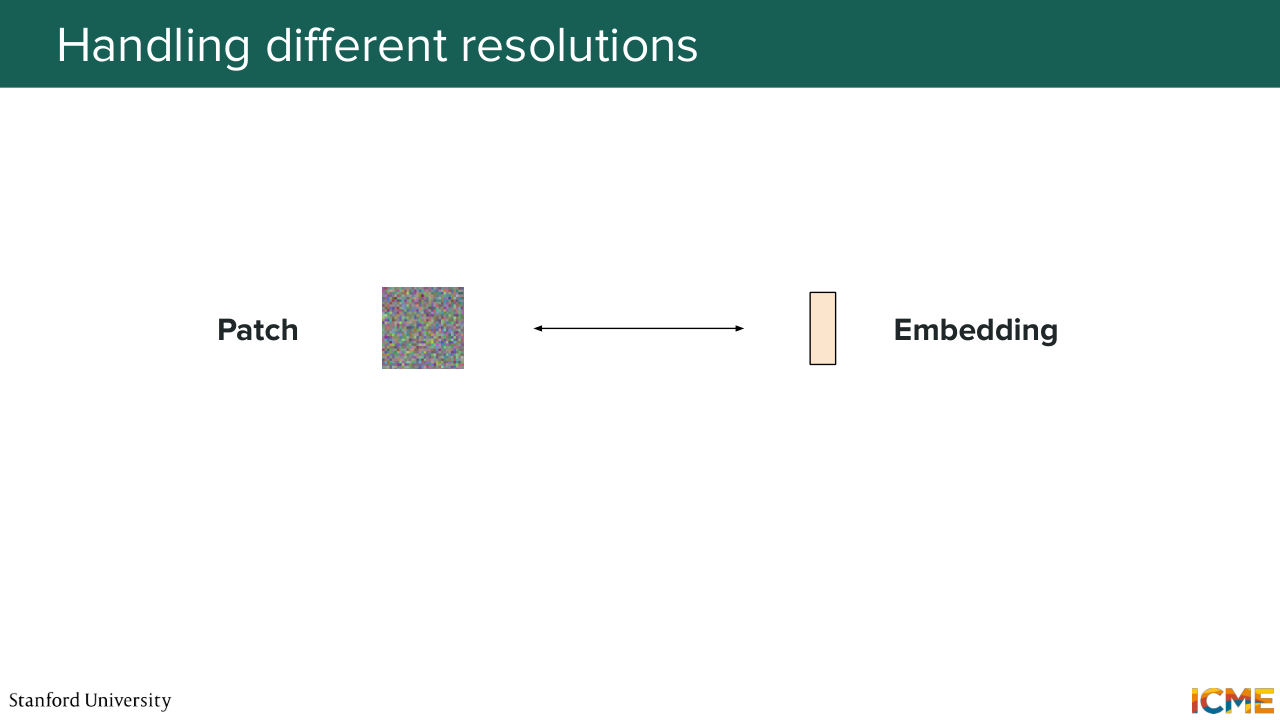
51:43 And so I want us to remember that the default architectures these days are DIT-based. And in DIT, what you do is you divide your input into patches where each patch is equivalent to some embedding. And so what happens is for low resolution, you will have a certain number of patches,
52:09 some number of tokens. And for high resolution, you will just have more tokens. Yes, exactly. So yeah, that's exactly that. It's as if it was large context. And if you remember the length t will be i, which is the dimension of an input. So if it's a squared over p squared. So that's the order of magnitude to have in mind. I will go ahead and move on to the second step of the training
52:43 lifecycle, which is the post training step. And so here what we want to do is
Shown briefly — discussed together with the adjacent slides.
Shown briefly — discussed together with the adjacent slides.
Shown briefly — discussed together with the adjacent slides.
Shown briefly — discussed together with the adjacent slides.
Shown briefly — discussed together with the adjacent slides.
Shown briefly — discussed together with the adjacent slides.
Shown briefly — discussed together with the adjacent slides.
Shown briefly — discussed together with the adjacent slides.
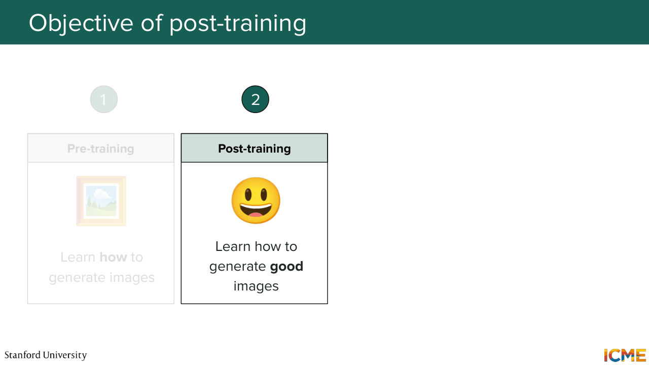
52:51 to teach our model on how to generate good images. Now you may tell me, "Well, what does good mean?"
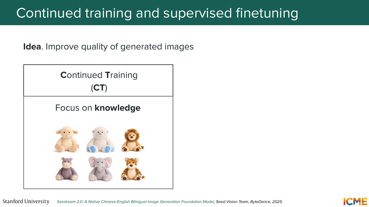
53:02 Well, you have, of course several angles, but I'll talk about two main names that you will see out there. The first one is called continued training, CT, which is around teaching your model on a bunch of other things that you may care about in your task of interest. So I'll give you an example.
53:28 So let's suppose you have a model that has been pre-trained on a bunch of nature images, and cars, and so on, but what you want to do is to have a model that generates images of teddy bear. Well, what you'll do here is you will have a dataset of what you care about, and here that is teddy bears. And you will just continue your training on that data set.
53:55 So that part, you can think of it as focusing on increasing your knowledge.
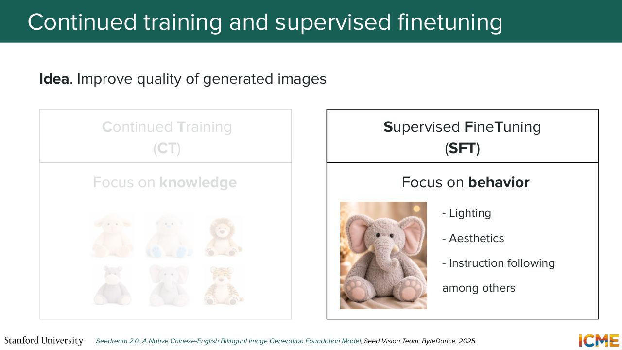
54:03 Then you have another category of post-training methods, which are called supervised fine-tuning. Same thing, but here the mindset is to focus on the behavior of your model as opposed to increasing the knowledge. So in that case, what that means is generating an image that is more aesthetically pleasing, that has better lighting, or that just follows the text better.
54:35 So these are the kinds of dimensions that you care about.
54:40 And up until now, we've only seen
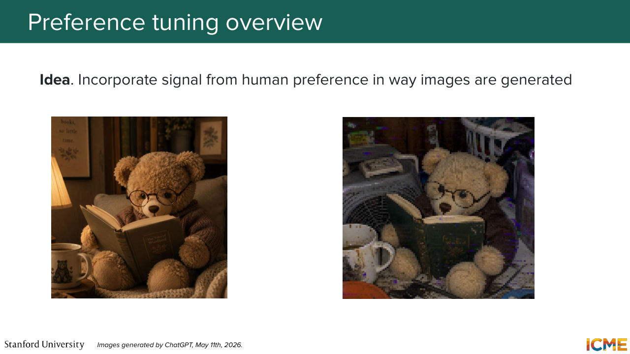
54:45 how to teach our model on what to do, but we have not taught our model on what not to do. And that is the objective of the second category of methods, which is preference tuning methods, where for a given prompt, you may have two images where one of those images is something that you want to happen more than another one.
55:14 So here I will illustrate an example of the left image, which is an image of a teddy bear reading, very high resolution, good lighting, and aesthetically pleasing, and the one on the right, which is not as aesthetically pleasing. And what you want to do is to incentivize your model to generate an image that is more aligned with human preferences.
55:41 So here the thumbs up and thumbs down are typically either human ratings or some measure that you can obtain with some model that we will talk about next lecture. But you will need to have some measure of pairwise comparison or listwise comparison of different images. And in this case, the left image being better than the right one.
56:10 So how do you do that? So before we move further, I just want to say that the field is still a developing field, and that next to it, there's also the text field, the LLM field, that has been growing. And so one observation is that you will find the same kinds of techniques that are used in the LLM space be adapted for the text-to-image generation space.
56:43 And that is something that I'm going to show you in the slides that will follow.
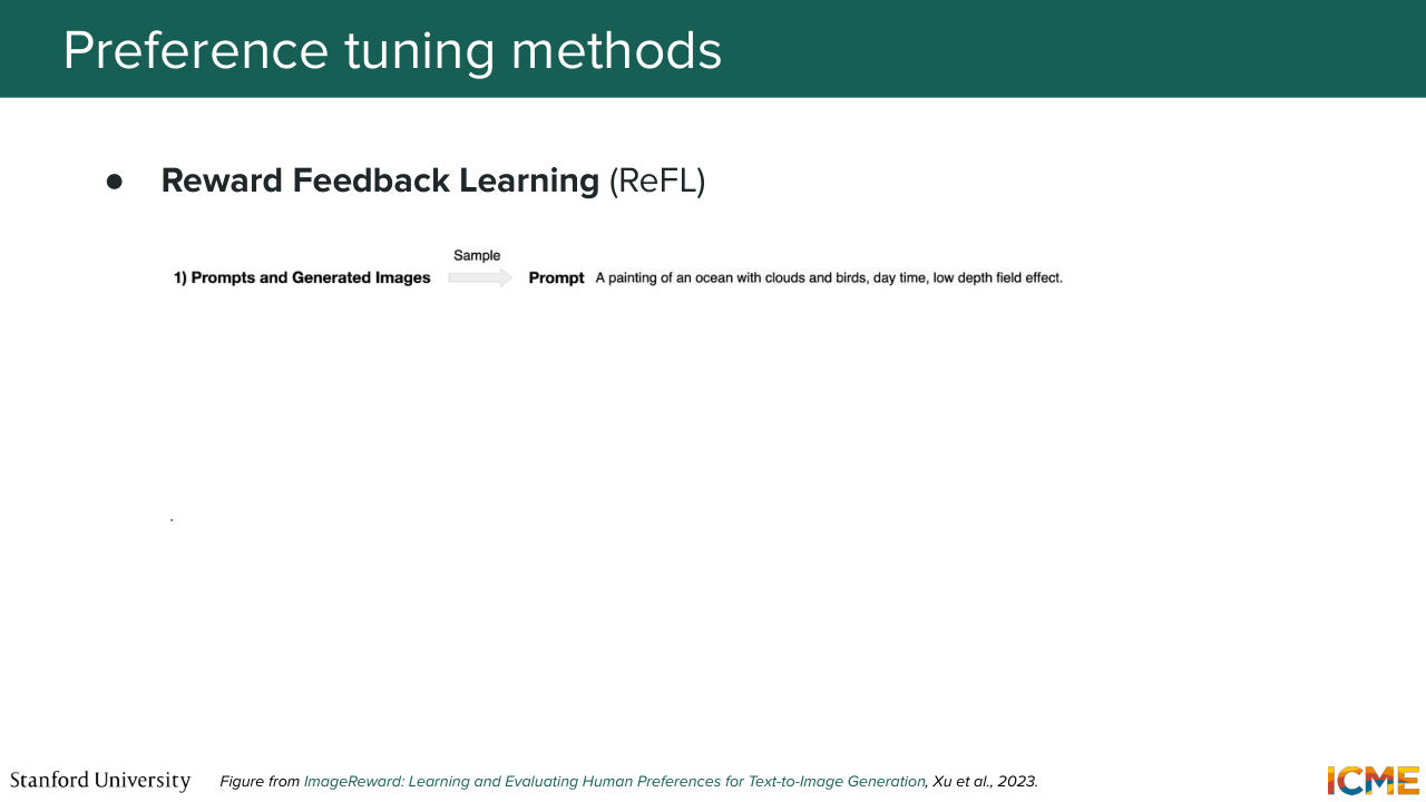
56:49 So the first method that is around tuning your model to incentivize generating images that are more aligned with human preferences is a method called reward feedback learning. So I'll go step by step into what that does. So as I mentioned, what you do is you take a prompt,
57:16 and then you have a bunch of images related to that prompt. And what you do is you try to get some sense of which one is better than the other. So you can either get pairwise ratings or even list wise ratings. So for instance, A is better than B, than C, et cetera. And from there, the idea is to train a reward model
57:46 that takes in a prompt and an image, and that gets you a score that tells you how good that image was with respect to the score, or how good that image was with respect to the prompt. And so here we will not go through the math. So in case you're interested, we actually have a whole lecture on that in our sister class, CME 295.
58:13 But long story short is that you can use a pairwise loss based on formulation called the Bradley-Terry formulation and train a model that does that for you. So at the end of this step, you get a reward model that takes in a prompt, that takes in an image, and that tells you how good that image was to this prompt.
58:40 So what you care about is to tune your text-to-image generation model to produce images that are higher rewards, because the reward model that you trained is something that hopefully aligns with human preferences. So if the reward model says that one is good, then hopefully, it's something that is aligned
59:09 with what the human would say. And what you want is to train your image generation model in order to produce images that are higher rewards.
59:25 So there is some math involved, but at a very high level, what we do is we take the noisy latent, we predict or generate an image for which we have the reward. But in this case, the good thing is that we have the model. We have the reward model. It is a reward model that we have at our disposal. So it is actually something that is differentiable.
59:52 And so here, you can back propagate the loss or the objective that you have, which is to maximize those rewards back into your image generation model in order to incentivize that model to produce images that are higher rewards. So that is reward feedback learning. The second method I will introduce
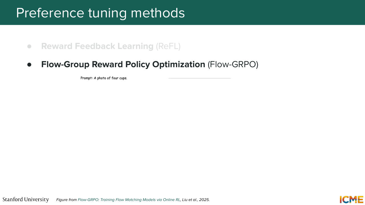
1:00:21 is called Flow Group Reward Policy Optimization a.k.a. Flow-GRPO. So for those of you who are also in the LLM field, you may have heard the term GRPO a lot during the past year or so. And so here, the idea is to leverage that algorithm in the case of image generation.
1:00:45 So in a very similar fashion, what you do is you take a look at images that are generated by your image generation model, and in this case, what you want is for a given prompt to have a diverse set of generated images. So it's going a little bit into the details, but the authors are framing this via an SDE
1:01:15 that increases the diversity of images that are generated,
1:01:21 so this is all so that we can have, for a given prompt, a diverse set of images that are generated. And from there, compute relative rewards, meaning you pass each prompt along with each image to some black-box reward model, and it tells you whether or not that is a good image. And what you do is you compute a relative measure
1:01:56 of how good that image was with respect to the other image in your group. So that's why this method is called group Reward Policy Optimization, is because you actually compute-- so an advantage, that's the technical term, which is the reward relative to the reward in your group. And then based on that, you update the policy which is your image generation model.
1:02:24 And so one thing that I want to say, and it's true for all of these reward-based approaches, is your reward is not necessarily something that is fully aligned with what you care about. And so you can have a problem of reward hacking, where your model is being updated too much in a way to optimize the reward that is not perfectly aligned with what you want. And so in order to have a way to mitigate that issue,
1:02:57 you typically have an extra term in your loss. And so here in the slide it's kind of small, but it's a KL divergence term between the policy that you're training on and the old policy. So it's just a way for you to not have iterations, updates that are too far from the old model.
1:03:20 And the last one I will mention, and here I'm
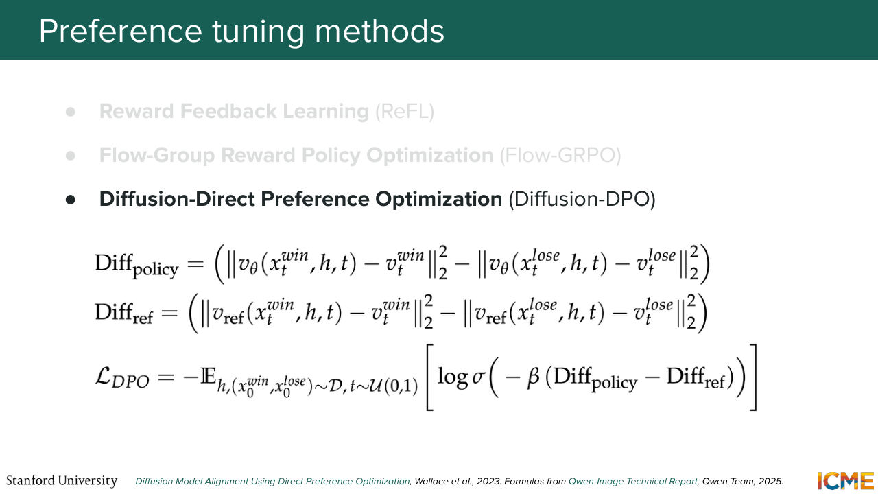
1:03:26 sorry for this big formulas, but I couldn't find a good illustration for this one. So this one is called Diffusion DPO. And Diffusion DPO is the diffusion equivalent of DPO, which is a supervised method used in the LLM world to tune the weights of your model with respect to human preferences.
1:03:50 And here, what you need to take away from these three lines of equations is that you want to incentivize your model to predict cities associated with "winning" images. You want to incentivize your model, doing a better job at predicting those, and you want to incentivize your model to do a worse job
1:04:18 at predicting velocities of the "bad" images. So if you do that, you're going to have a higher chance of having the winning images be generated and a lower chance of having your model generate the worse images from being generated. Does this part make sense?
1:04:41 So we have these three lines of equations. You can stare at it after the class. It's something that also tells you that we want the model to be better at predicting velocities of winning images, and worse at predicting loss velocity of losing images. So yeah, so this is what this loss is telling you to do. OK, great. So there is one last thing I want to tell you.
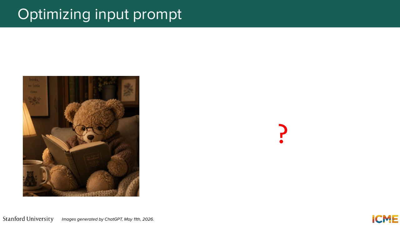
1:05:10 We want to make our images better. And I want you to tell me, or I'm asking if you would know what kind of prompts
1:05:23 would lead to that kind of image at this point in time, in the training, if you were to guess. So here on the left, you have a beautiful image of a Teddy bear reading a book. So the question here is what prompt do you want to put? Anyone wants to try? Can be creative.
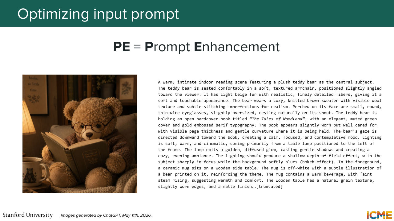
1:05:52 You think it's a trick question. So I'm going to just for the sake of time, tell you what the prompt was. So it's actually a truncated prompt, and I'll just read the first few words. So "A warm, intimate indoor reading scene featuring a plush teddy bear as a central object, and it talks about how the objects are, how the lighting is."
1:06:14 And it's actually maybe four times what is on the slide. So the point here is that these alignment methods allow us to have much greater control on what we want the output image to be. And there is, therefore, a mismatch between what we teach the model and what users tell to the model. Because let's be honest, you and I,
1:06:44 if we want to create an image of a teddy bear, we'll just say "a teddy bear reading a book." But we want something that looks like this. So there needs to be something in between that is able to prompt our model well in a way that will generate beautiful images. And there is a method called prompts enhancement, which
1:07:08 will take a given user input and transform it into a very elegant, long, detailed prompt that would be similar to the kinds of prompts that the model has been trained on. And so this is all for us to have a beautiful image based on a prompt that is in distribution, if you want, and that is leveraging the capabilities of the model. So I just want to take a pause here.
1:07:39 So I know I'm doing a lot of metaphors comparisons, but let's try to recap all the steps we've been through
1:07:47 by taking the following analogy. So let's assume that our image generation model is us, is similar to us actually learning how to cook. So pre-training is about learning how to generate images. So here just learn about the different kinds of foods. Post-training is about learning how to generate "good" images. So here, what does good mean? So these are examples that we give you, so supervised fine tuning and continued training.
1:08:21 Continued training is new knowledge. So here, it's as if I was reading about recipes. So I read about recipes of how to make good food. And then supervised fine-tuning is about the aesthetics, it's about the prompts, the instruction following. And so here, I'm just making sure that the food looks great. The delivery is good. And then you have the preference tuning stage where you want to make sure to do more of the things
1:08:49 that you may like rather than not. And in this food analogy case, you have an inspector, food inspector that comes, and you cook several times the same dish. And inspector just tastes how good each of the dishes that you prepared was and it just tells you which one was better. And you update your way of cooking based on that. And this prompt enhancement thing is the same as you being
1:09:21 in a restaurant and a customer walking in and telling you, "I want meat." But for you, you just know medium-rare kind of meat with a pinch of salt and so on. So you will have a waiter between the customer and yourself that will rephrase the customer's request
1:09:48 in a way that aligns with what you have learned. And this is exactly what prompts enhancement is. I hope this made sense. And with that, let's go to the third stage of the training
1:10:02 lifecycle, which is tuning. So as I mentioned, tuning is about personalizing your model for a special use case that you care about. And so here, the method that I want to talk to you about
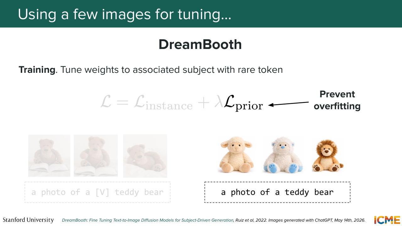
1:10:20 is a method that you may have seen on the internet because a lot of people have been using it. It's called DreamBooth. And the idea is that you have something of interest, let's say a specific teddy bear, that you want to have in the images that you generate. You don't want any teddy bear. You want that specific teddy bear. So what you want is to personalize your model
1:10:53 to generate images of that very specific teddy bear. So here's what you would do. What you would do is taking your model and then having a few images of that very specific teddy bear that you have, take images of that teddy bear with different poses, and train your model to generate that teddy bear based on a prompt that relies
1:11:23 on a rare token, that is here bracket V. That will teach your model to associate that specific person/object reference with that token. So you do that. So let's say you do that. Do you see an example or something that can go wrong.
1:11:52 If you train your model to generate these images based on that prompt? OK, let's assume you just do that. Yep. So the answer is it's not diverse enough. So I think you're very, very-- you're touching exactly the problem that we have at hand, which is that you will
1:12:18 specialize your model too much into generating that and actually forgetting the kinds of concepts, the kinds of images it was able to produce before. And so for that reason, so it's a great answer for that reason, what you want is to also make sure that your model does not lose the ability that it had before. And so that's why what you would want to do is to have some reference of text-to-image pairs that it was able to generate
1:12:49 successfully, that you would also tell it to generate successfully and combine the two into a loss that tells you, "I want to generate images with that specific teddy bear, but also preserving the performance that I had in the past." And this is called the prior preservation loss. That's second term.
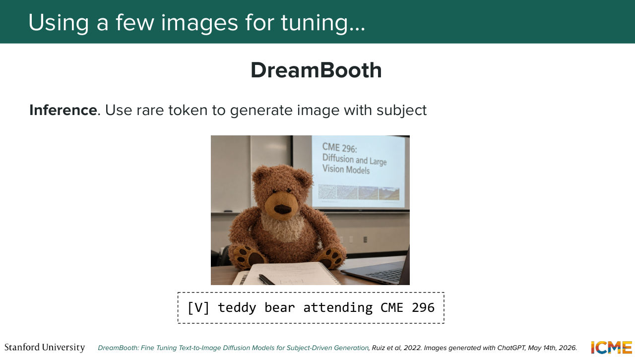
1:13:15 So when you do that training-- and so yeah. So you prevent overfitting. So when you do that training, what you're able to do is to use that rare special token that you have trained your model on and then generate new images in specific settings. So here the special token teddy bear attending CME 296, so this is how teddy bear would look like. So that method is great, and what we're doing is updating our model and in particular the model
1:13:50 weights in order to reflect what we want to generate. Well, the problem is your model can be quite big. It can be as big as billions of parameters. I believe the biggest text-to-image models that are out there are in the order of tens of billions, the open-source ones. And so you would not want to update all the weights, which
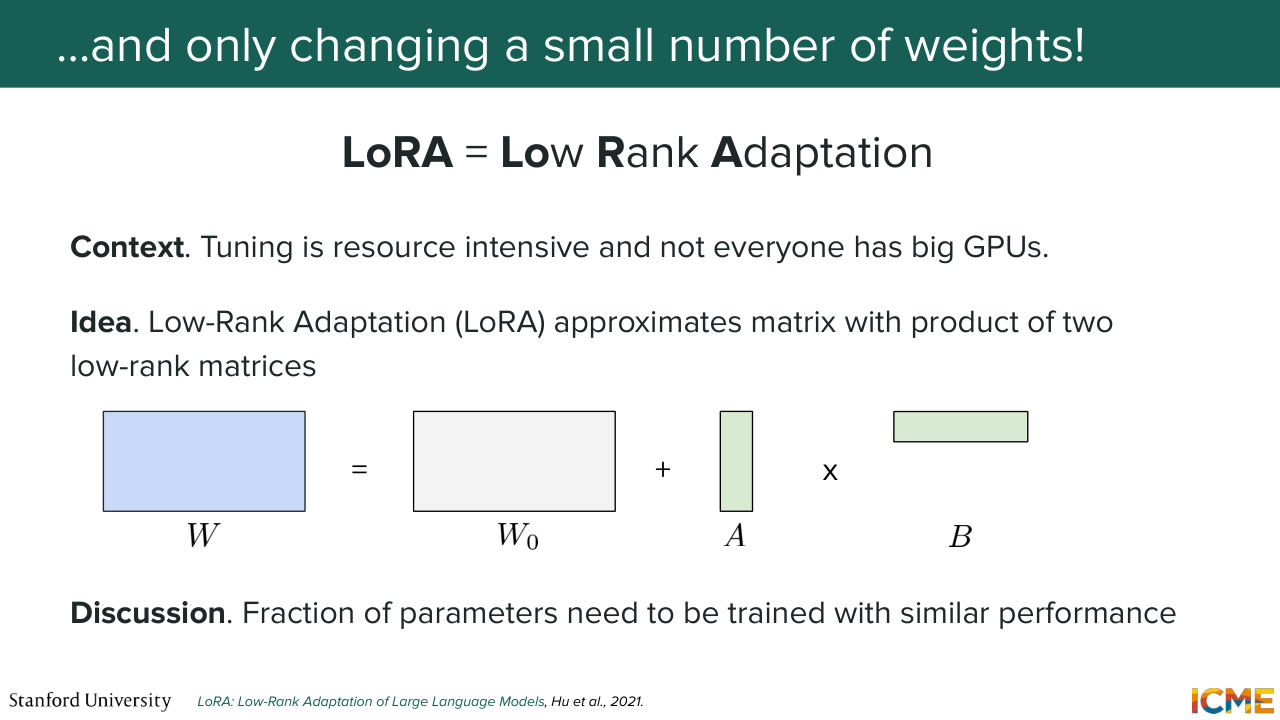
1:14:19 is the reason why there is a method that is very commonly used in the LLM world, which is also something that people use in this instance, which is called LoRA, and stands for Low-Rank Adaptation. And what this method does is instead of training all the weights of your model, what it does is it only trains a fraction by considering
1:14:50 that the weights of your model are the weights of the base model, plus two low-rank matrices. And the reason why it's called low-rank adaptation is because it leads to A times B, that is low rank. And so when you do that, it turns out that you can preserve most of the performance but train that with a fraction of the cost. So you will see methods that are called "DreamBooth + LoRA."
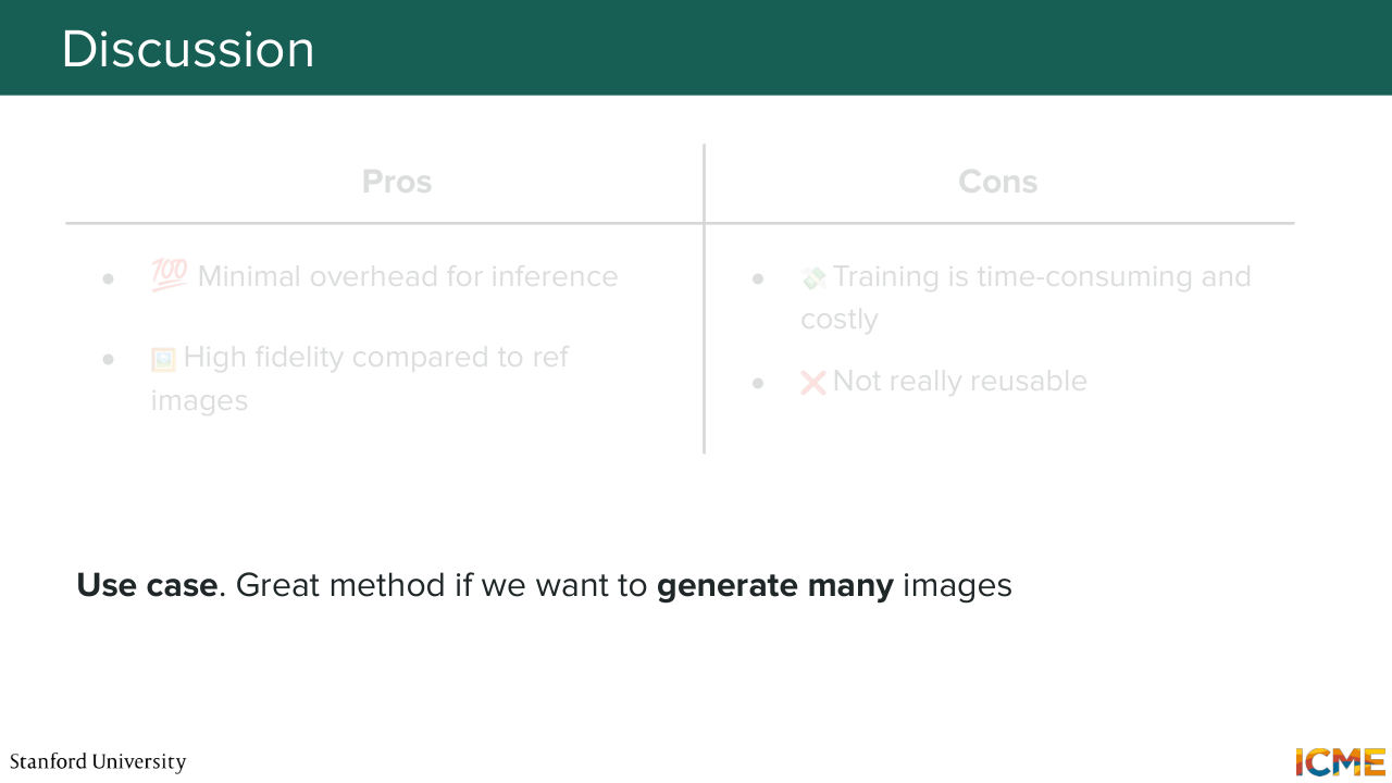
1:15:19 And that is what it is about. And I want to talk about the pros and the cons of this approach. So the pro is-- the good thing is if you want to generate thousands and thousands of images of your teddy bear, well, you can do that. And the results are pretty high fidelity. They match pretty well the details that are in the input images.
1:15:46 But the con here is if you need-- or if you need to do that for a lot of special cases, well, you need to absorb the training costs, which is pretty time consuming and costly. And also, it's something that you cannot really reuse if, for instance, you want something else in your images.
1:16:10 And I would just conclude by saying that this approach is great if you're in a use case where you need to generate many, many, many, many images of one specific subject, or person, or object.

Shown briefly — discussed together with the adjacent slides.
1:16:31 And with that, I'll give it to Shervin.
Shown briefly — discussed together with the adjacent slides.
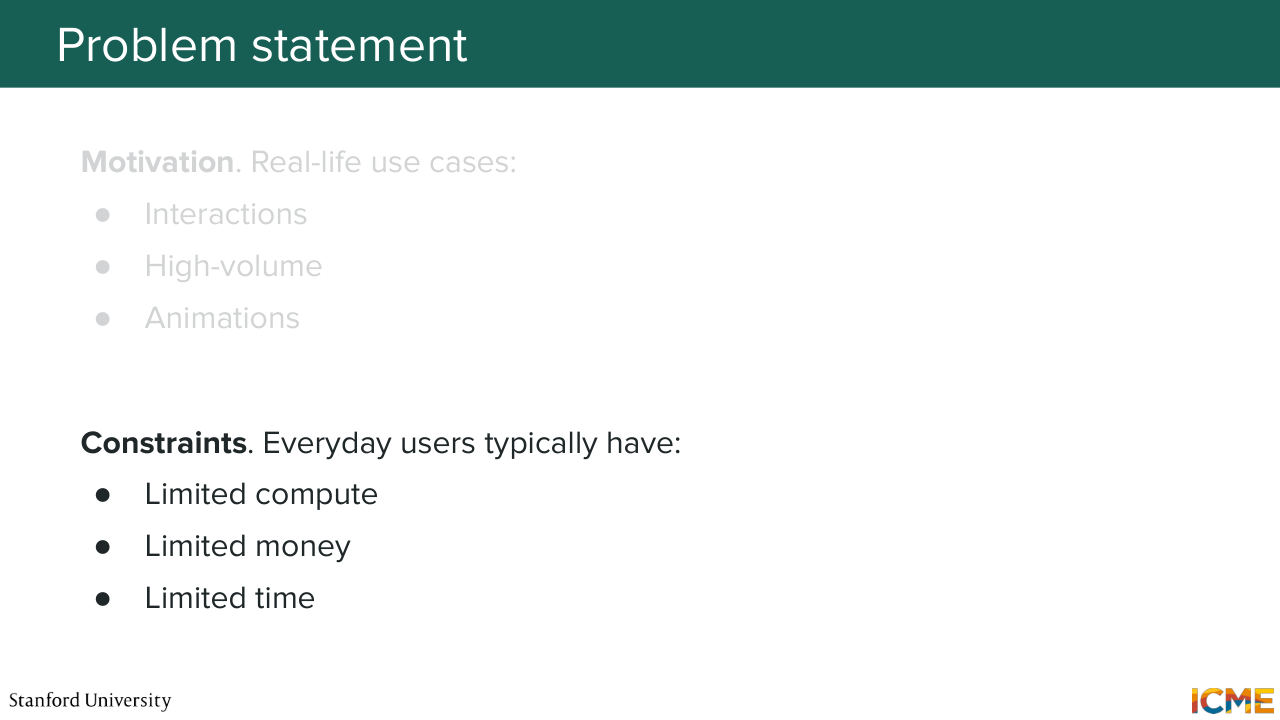
1:16:36 Thank you, Afshin. So we're going to continue together on that note of efficiency and looking at distillation techniques which aim at preserving some of the high quality that we were able to develop with these models, but at a lower cost. So all of these methods produce state-of-the-art images,
1:17:00 but in real life, you might be a user that uses a service that is high volume. So the provider doesn't have an incentive to spend a lot of money on each query. So you don't want typically to have 1,000 steps to generate a single image. Similarly, if you're in a business setting, you want to achieve a given goal, and your goal is not necessarily to be the best, but just good enough.
1:17:28 And then that trade-off between good in terms of quality and cost is something that you're going to be interested in. And then you can cite other applications where real-time properties are important. So this is why it's worth investigating techniques that are fast. And then all of these are, of course, linked to properties
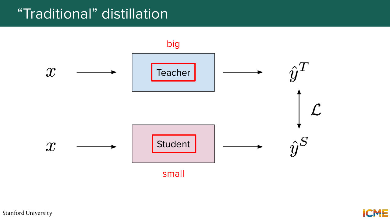
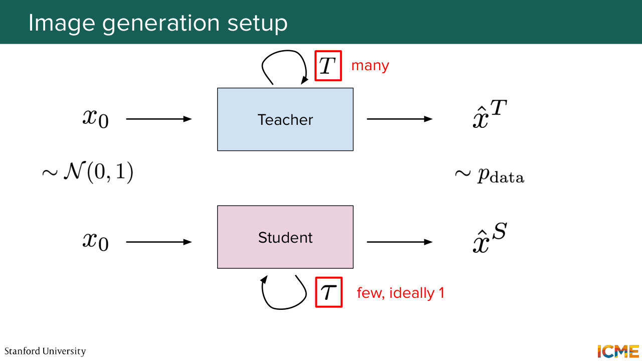
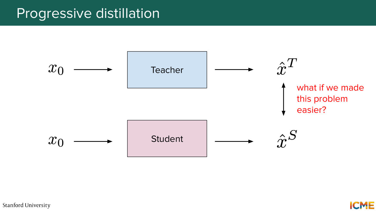
1:17:52 that we care about as everyday users. So we don't want to spend a lot, and we don't want to spend resources inefficiently. And if I was to tell you about distillation in the traditional world-- so you would typically see something that looks like this. You have a teacher model that is big and a student model that is typically of a smaller size.
1:18:23 And you both want to predict the same outputs. And here, for example, so I'm borrowing these slides from CME 295, where we wanted to distill some of the knowledge on next token prediction. So what is important in this distillation technique is truly the shape of the distribution that is learned. And you can see that you can get away with smaller models, directly anchoring on it and then
1:18:54 producing a level of quality that is almost just as high. So just to give a quantitative example, you may think of a BERT and DistilBERT, where you save quite a bit, I think 60%, half of the parameters, roughly, and you retain 97% of the performance. So this is something that we are interested in doing as well here. So in the LLM world, for example,
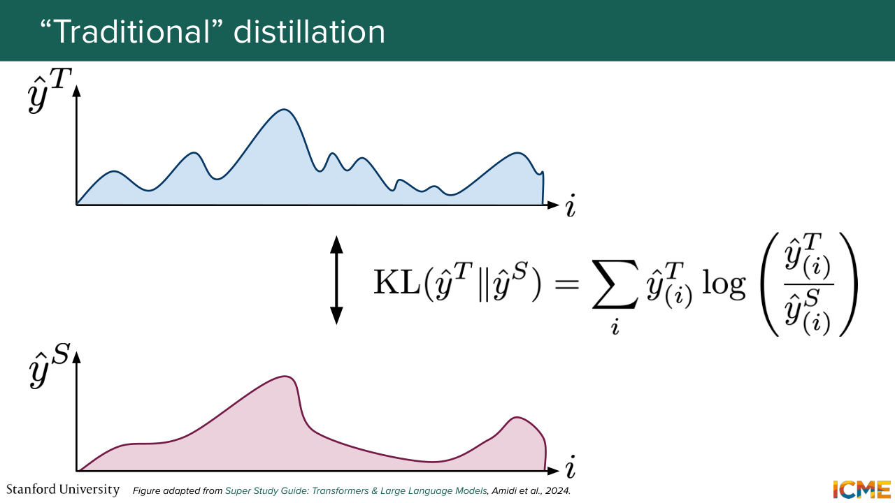
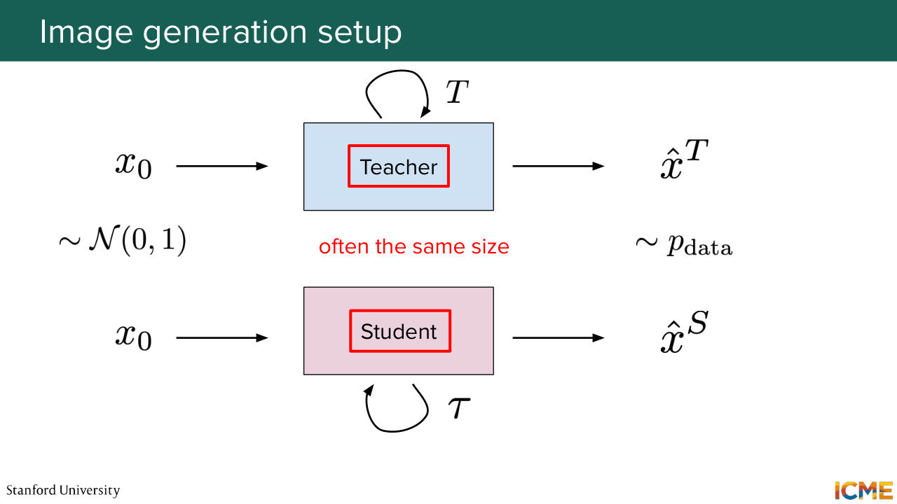
1:19:22 you would do so with the KL divergence between the two. So here, the loss says if we assume that the teacher distribution is a true one, how bad is it to approximate it with a student one? And this is how you perform your loss optimization process with that kind of mindset. But here in the image world, well, you can try to reduce the size of the student model.
1:19:51 And it typically leads to much worse quality. And then you have another knob that you have as a low-hanging fruit that people typically tune, which is not the model size but more the number of steps. So you might remember from the first lecture that, for example, in diffusion you have, let's say 1,000 steps. Similarly, in the flow matching setting that afshin mentioned,
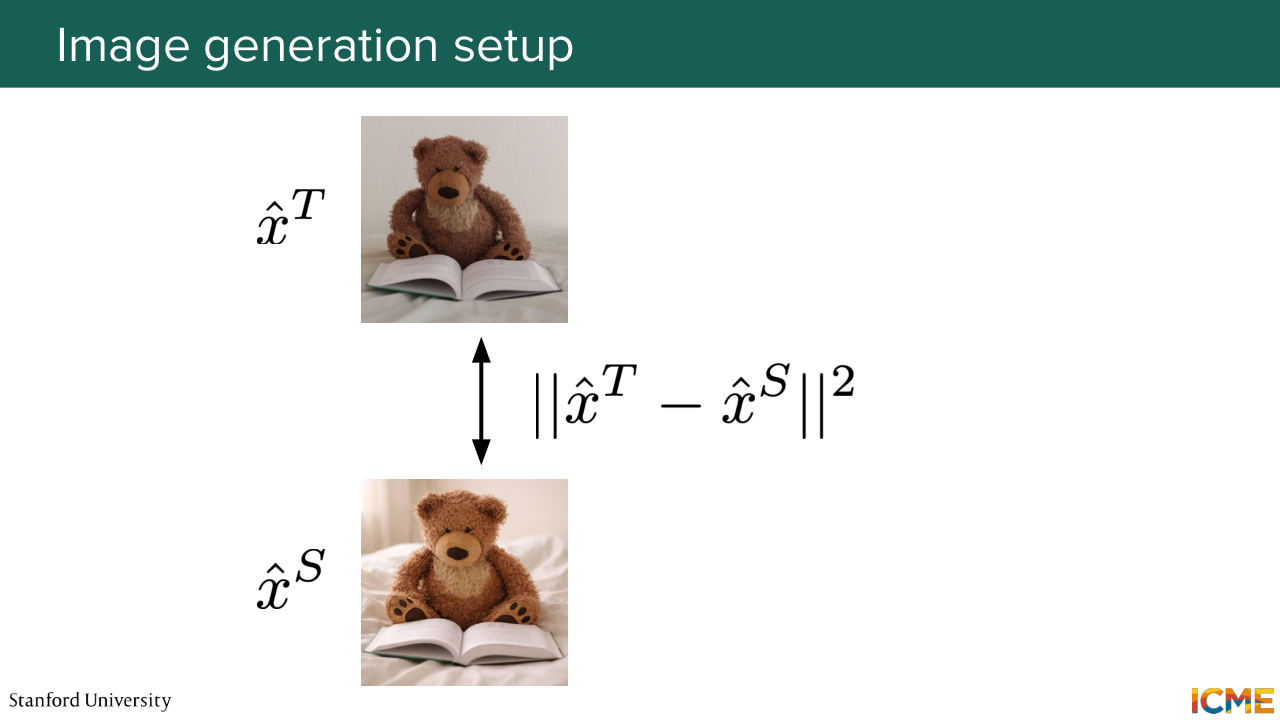
1:20:19 we were considering here, you typically have more than one step. And you would want to make it one, so that just a single pass gives you what you want. So here, we were not going to be doing typically KL divergence between distribution over tokens, but these kind of loss that regresses the output with respect to the teacher output
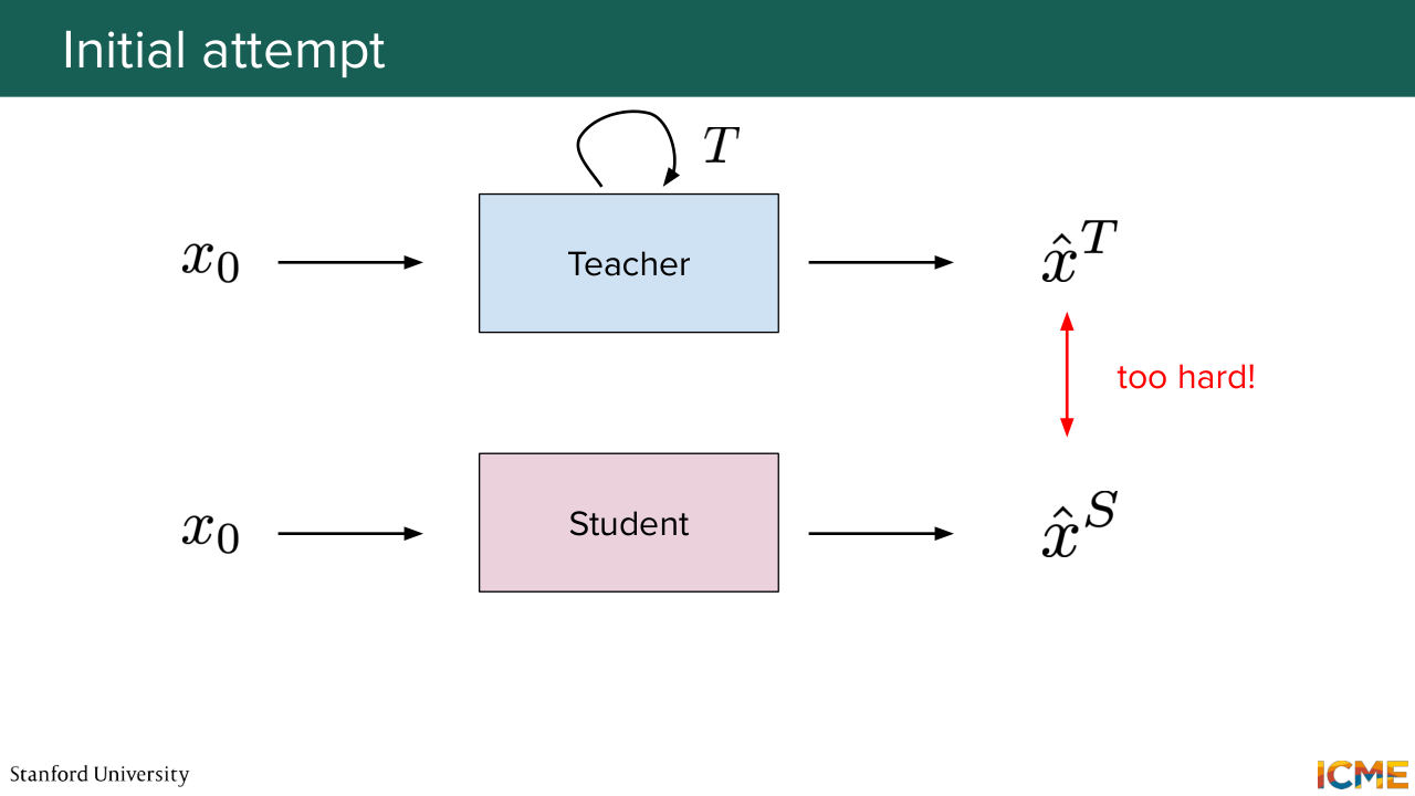
1:20:44 is something that you are going to see. So one way of doing it is with the mean squared error. We're going to see other techniques as well. And I just want us to do this thought exercise of approximating in one step directly the teacher output. So the issue is that it's too hard because you can--
1:21:12 so just to take the analogy that Afshin was taking last week regarding the painter, it's as if you ask a painter to paint a beautiful piece of art and then ask the students to do exactly the same with a single stroke. So it's way too much information packed for a single forward step to capture all at once.
Shown briefly — discussed together with the adjacent slides.
Shown briefly — discussed together with the adjacent slides.
Shown briefly — discussed together with the adjacent slides.
Shown briefly — discussed together with the adjacent slides.
Shown briefly — discussed together with the adjacent slides.
Shown briefly — discussed together with the adjacent slides.
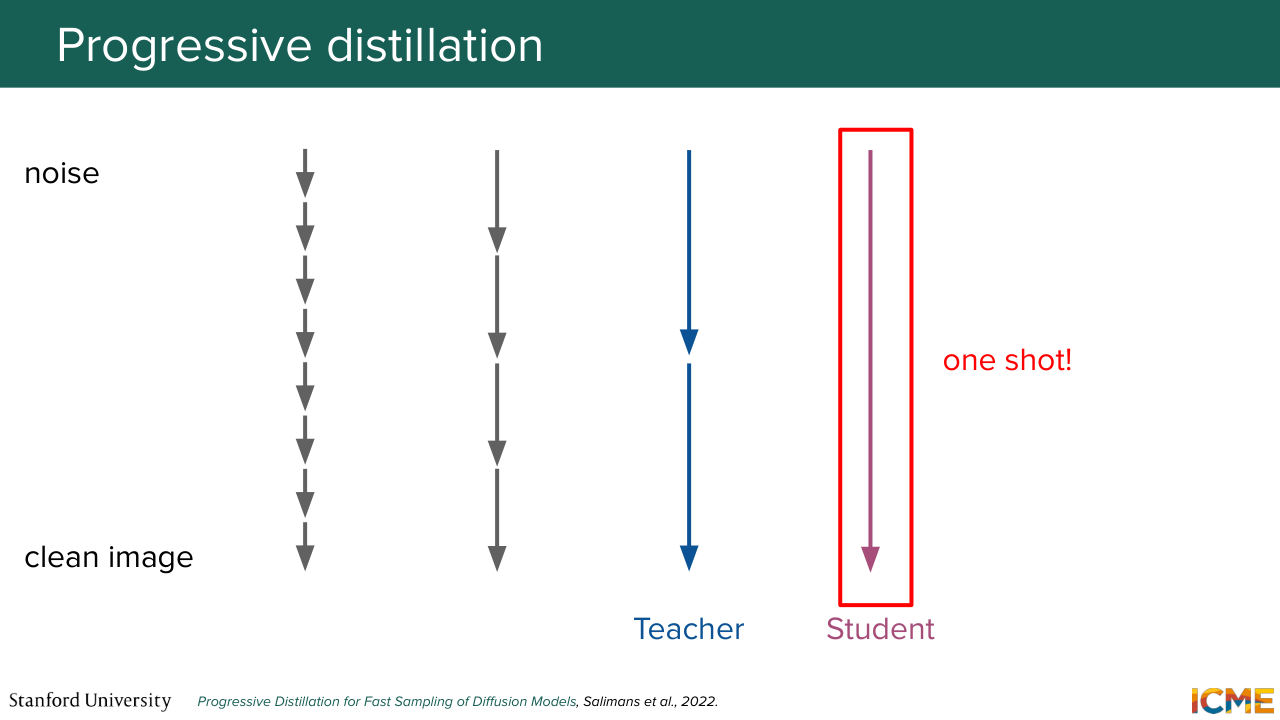
1:21:37 So you need a more granular subsequence of steps intuitively.
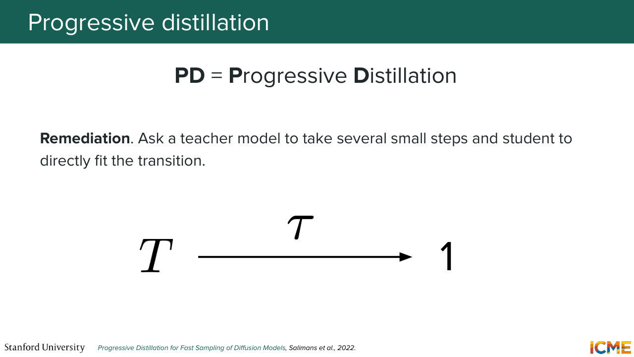
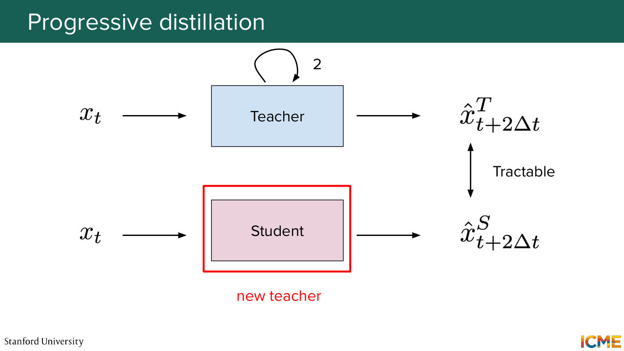
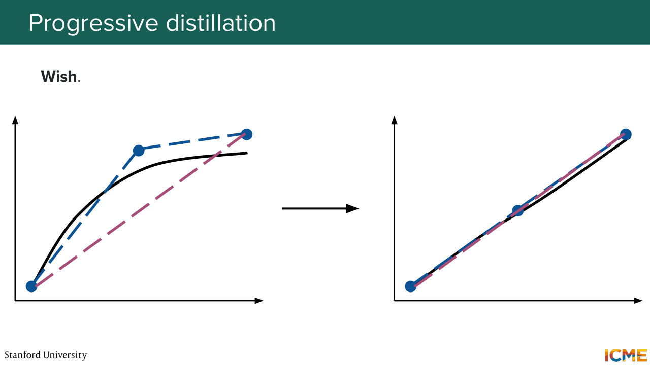
1:21:42 And this is what the spirit of progressive distillation is, where we take steps and ask the students to work on problems that are of approximate constant difficulty, and we iterate until we have a model that does what we want. So in other words, the formulation here is that we want the number of total steps to go from big T to 1. So here the method is as follows,
1:22:18 every time you try to do what you were doing in half the number of steps.
1:22:24 So I want you to make a thought experiment for a second between Afshin and I
1:22:30 and not suppose that we are twins, but instead, we are a tuple of size
1:22:36 n of identical brothers, more precisely of size log2 of number of steps. And here progressive distillation would be Afshin, for example, being the master painter for the first step. And every two strokes I would paint one stroke, and so on. And then once the process finishes, I would be the master painter, and then
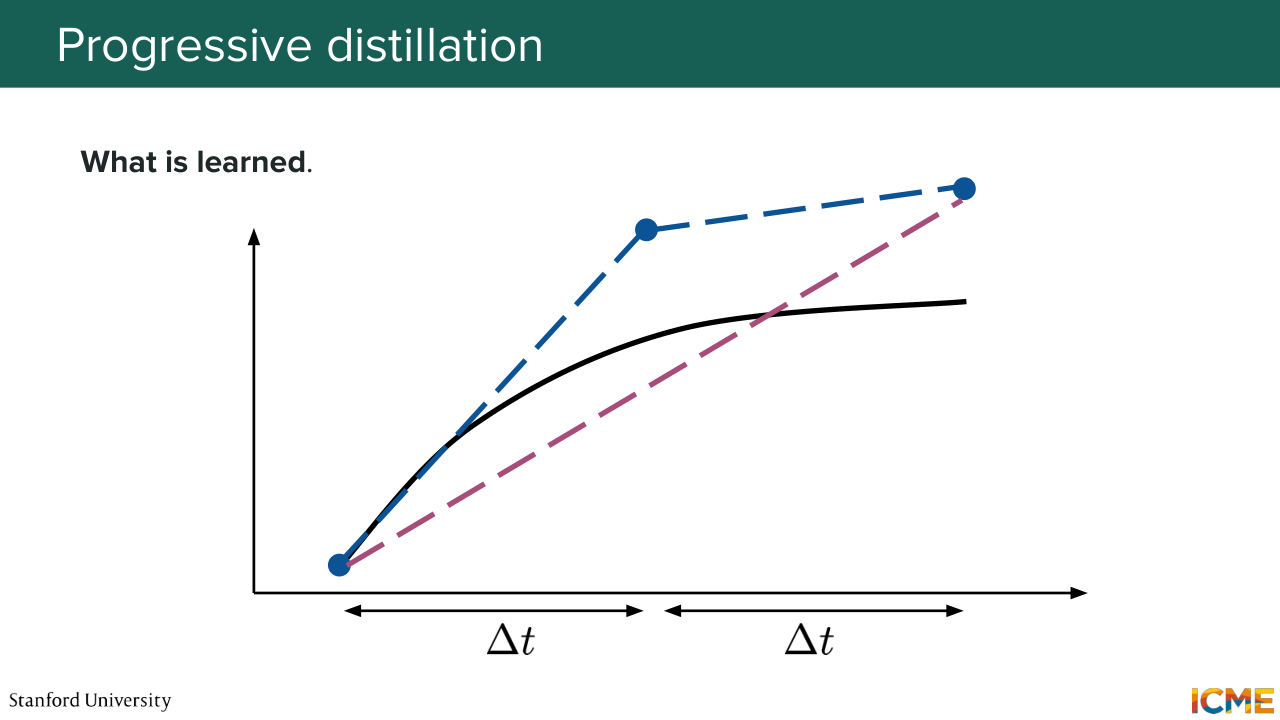
1:23:05 the next identical brother would be the student. So every two strokes that I paint, he would paint one stroke, so that at the end, you reach what you want in a single step. So just to give a visual representation of what we have learned here-- so you can see this as secant lines
1:23:32 that you draw in the space at every halving of the number of steps, which is a simple problem
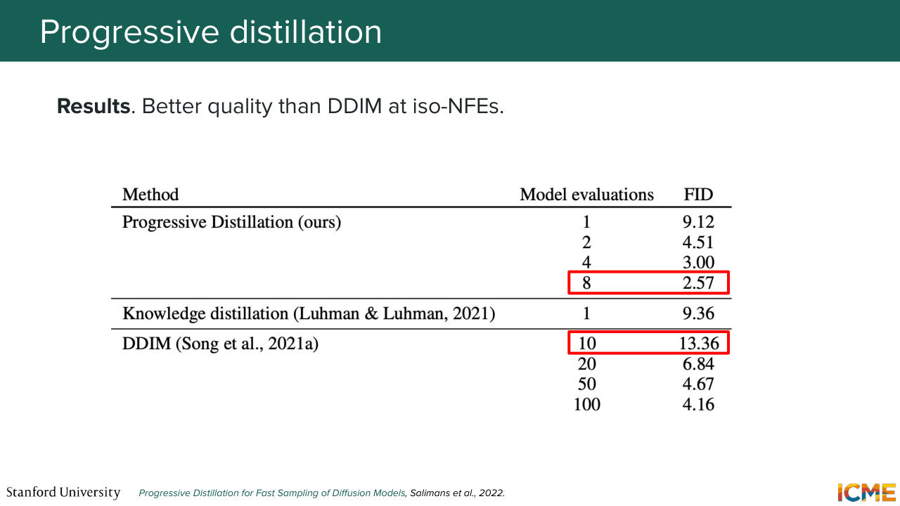
1:23:40 to take in isolation. And then when you do that iteratively, you reach the end goal. So looking at the results here, the good thing about this technique is that you can select the number of function evaluations that you're ready to spend, and you have an association with the end result.
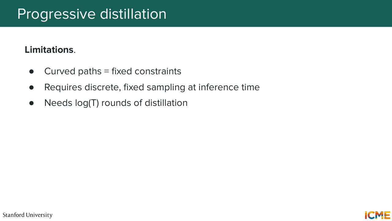
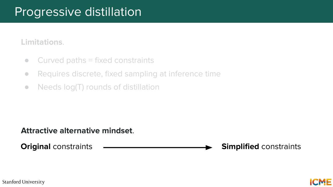
1:24:06 So of course, if you spend more steps, you're going to have better quality, but you have this level of granularity. And you see that you typically have better performance if you were to compare an equal number of steps, for example, in a deterministic technique like DDIM, like we had seen in the first lecture, which is nice. But here, one thing that we're doing
1:24:32 is that no matter how hard the path to getting to the clean image is, we're just taking it as a given. We're not saying, OK, let's to make the problem simpler.
1:24:45 We're just taking the problem as hard as it is and we're trying to work around it. And if you recall the third lecture on flow matching, there is something that we wish for that we might be able to realize, which is the reflow technique that helps in straightening paths in the space. So maybe we could make use of it. And this is what the paper called "InstaFlow" does.
Shown briefly — discussed together with the adjacent slides.
Shown briefly — discussed together with the adjacent slides.
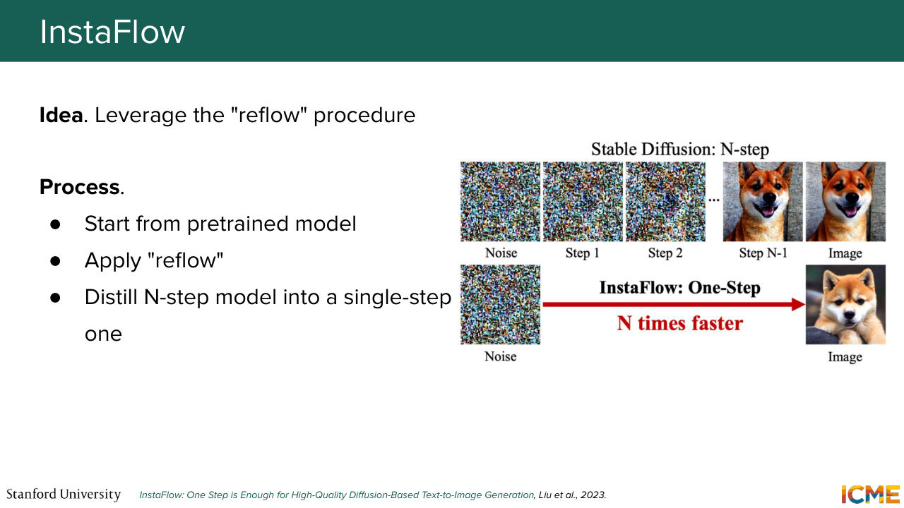
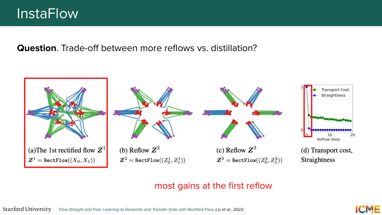
1:25:18 So it follows up on this idea of rectified flow that we had seen at the third lecture. So it does apply this method. And then on top of it, it adds a layer of distillation to further solidify the fact that we can get to the results in a single step. So just to give you a recap on what reflow was, so you had--
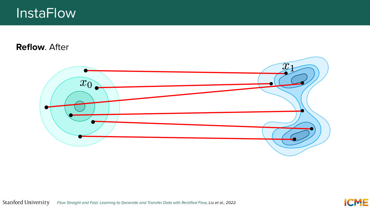
1:25:48 so let's say you sample from the easy distribution and then you integrate your ODE to get to the sample. Then you take these pairs of input-outputs and then you fit a new model, like a new model in it. And what you get is straighter path, typically, which allows you to take less Euler
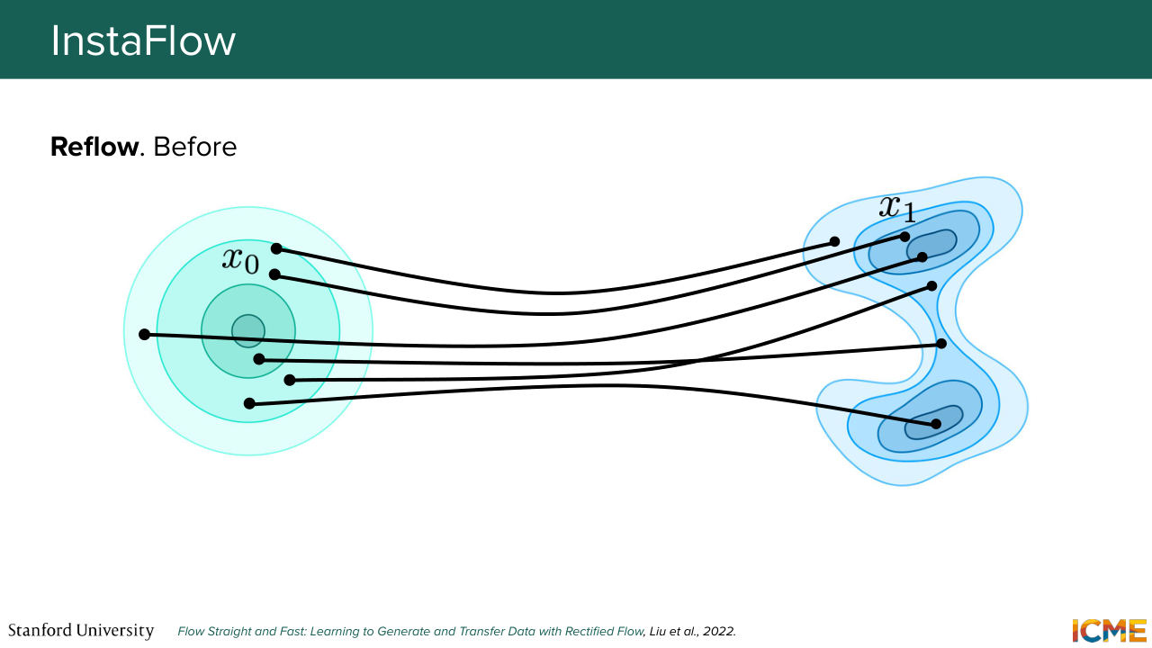
1:26:08 steps to get to the answer. But I have a question for you.
1:26:16 Let's say the problem is not totally straight, would you be inclined to do more reflow steps? 1:26:31 So it's a trick question. So the answer is if you do more reflow steps, then you introduce discretization errors
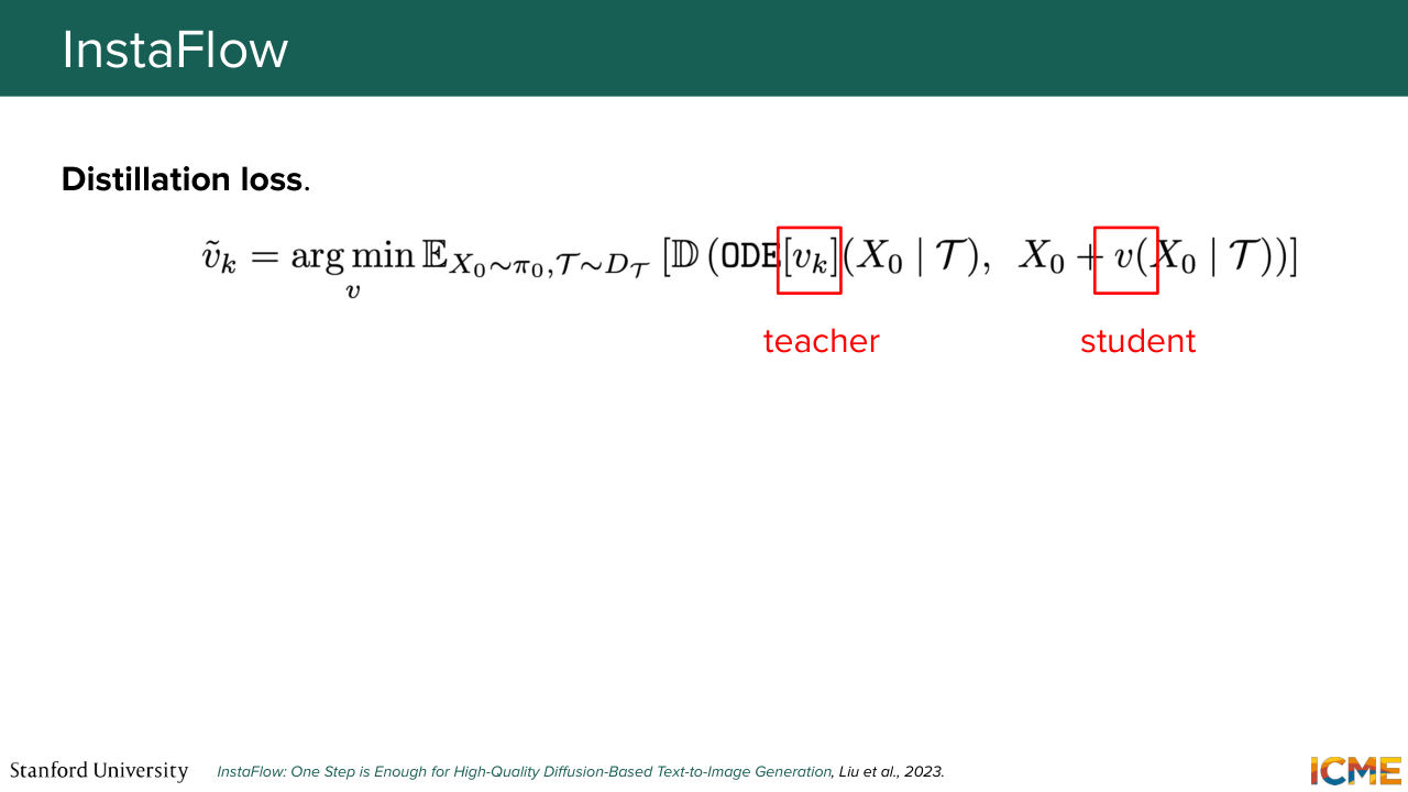
1:26:38 in your pairs. So the answer is typically no. And this is why what is pretty convenient to do is to give the task of still integrating that ODE to some teacher model and then have a student fit directly on that output. So this is what the distillation step does.
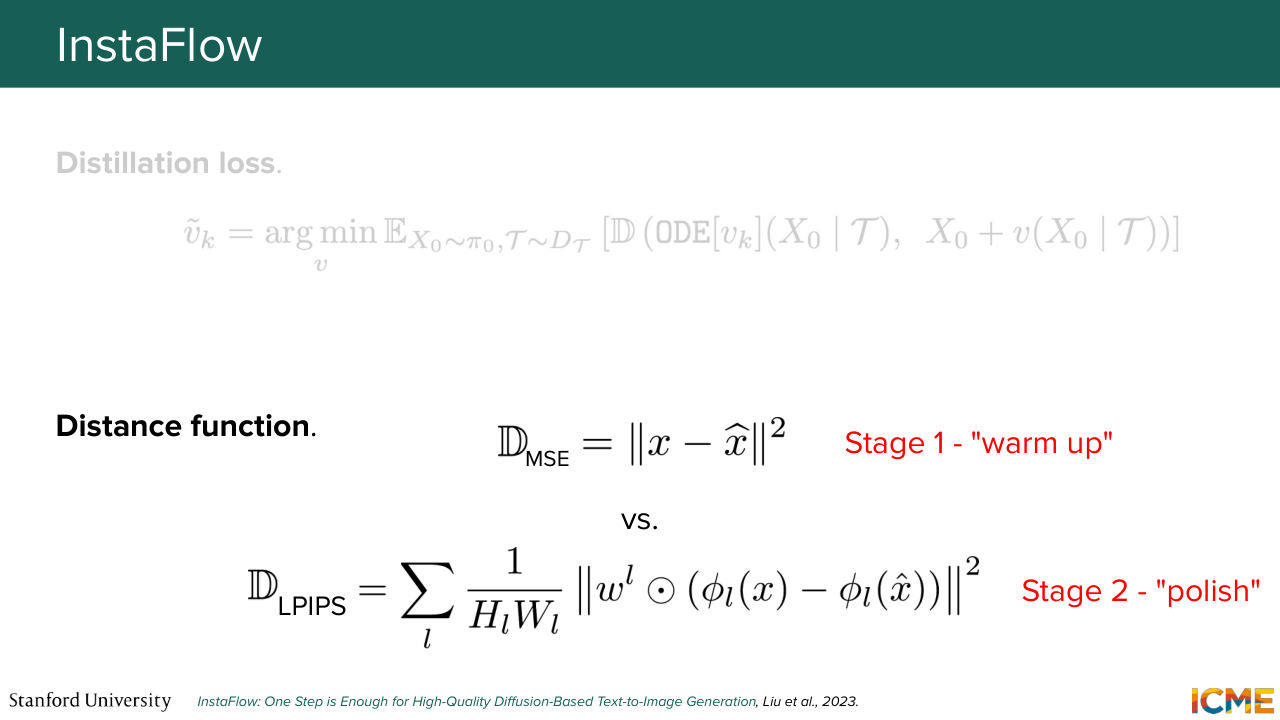
1:26:59 And then one interesting fact is that we use-- so this concept of distance between what the teacher predicts and what the student gets to. So you have this concept of warm-up, of using a simple distance metric like MSE. But we have seen in the previous lecture that MSE is not great to give a meaningful interpretation into whether the quality of the image is good,
1:27:27 because it focuses on the specific value of each pixel instead of the meaning of the feature, which is why this method uses the second loss formulation called LPIPS, Learned Perceptual Image Patch Similarity. And here, you make the image pass through a pre-trained model
1:27:54 with frozen weights, and then you compare the L2 distance between the feature maps instead over L layers. And this is what we just said.
Shown briefly — discussed together with the adjacent slides.
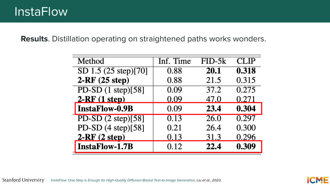
1:28:06 And then you see in practice, that the first reflow step gives you most of the straightening behavior, so you meaningfully-- you do not have an incentive to do more of them. And in terms of results, you see that you exceed the performance of whether-- of the fact that you add this additional distillation step
1:28:33 is better than just doing a reflow and having a single step. So it's the InstaFlow 0.9B versus the line just above that shows that. And yeah. So one thing that is tough with InstaFlow is that every time you do a reflow, it's an expensive process. So you need to do some pre work, which is--
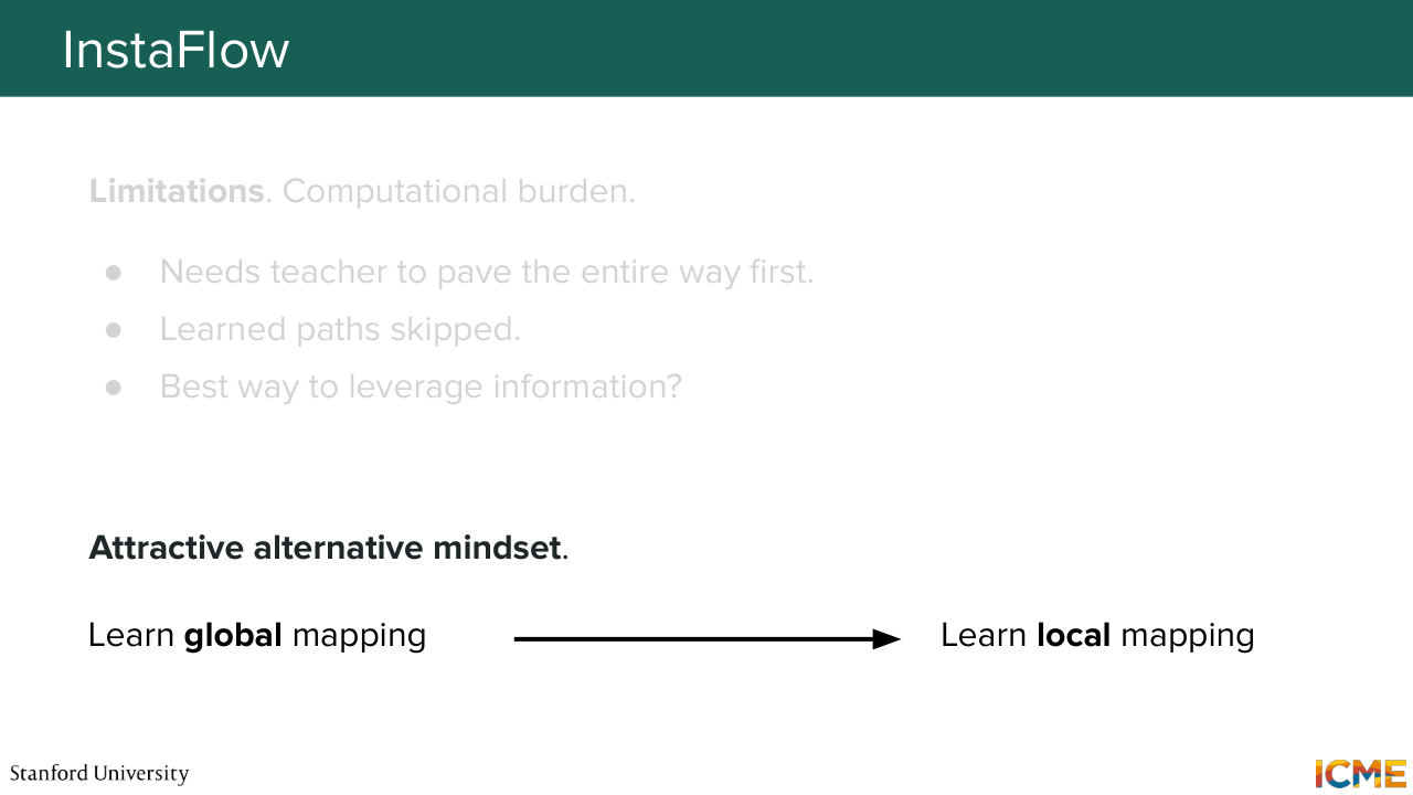
1:29:01 like the cost you have to pay here. And we're wondering if there is something we could do better when it comes to the path that are drawn. Is there some information that we could give to the student instead of making the problem simpler from the first place? But before I move on to the next mindset that I wanted to mention, I just wanted to pause for a second
1:29:27 and see if there is any questions. Yep. The question is, Why wouldn't you force straight path in the pre-training? You already do that, because you select a random noise at random and then a target point, and then you draw a straight line. But the thing is, these pairings, they're not optimal. So when you sample randomly-- and then the fact that you don't have these straight lines is not an intended design, but it's
1:29:55 a consequence of this MSE loss. So the reflow procedure is our way to remedy that, and there is no way to do that as early as the first train. OK, awesome. So I'm slightly late-- so I'm going to go through this next idea of leveraging
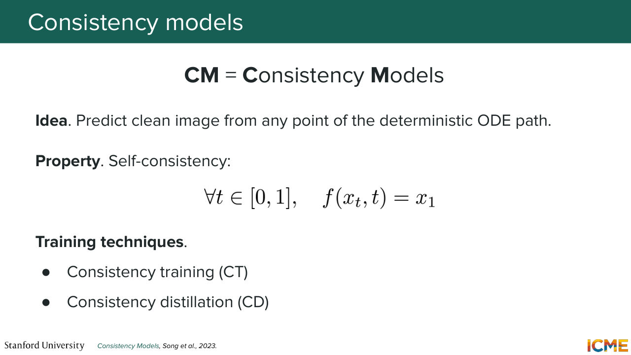
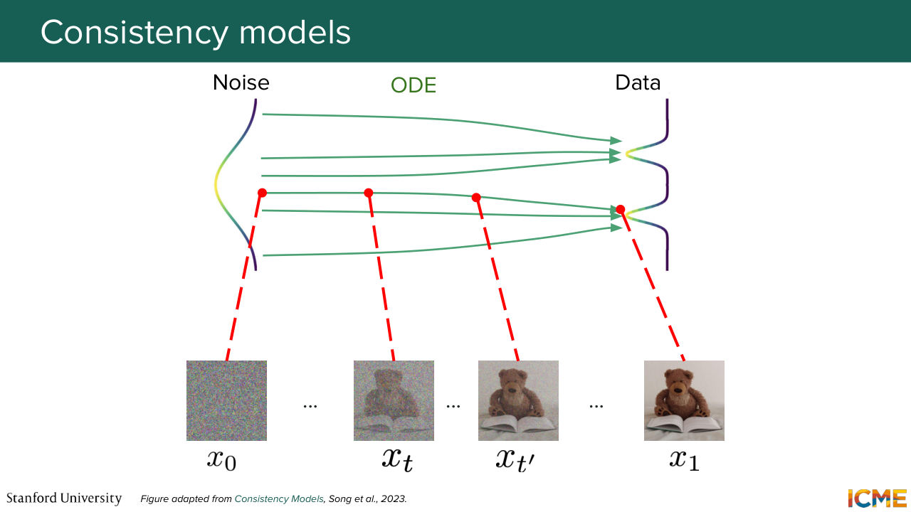
1:30:25 local properties to train a better student with this notion of consistency models, which has an interesting property of looking at paths that are deterministic with a mapping that maps every point of that path to the end goal, such that no matter where you are on that path, if you train your model to predict the end image, then you can make the jump as early
1:30:56 as when you are in the noise in the noise distribution. So just putting a picture here with our teddy bears and the flow matching case, if you have such a property, then every point on a given green line would map to x1.
1:31:21 And the way to do so is twofold. So you can either do it with so-called consistency training,
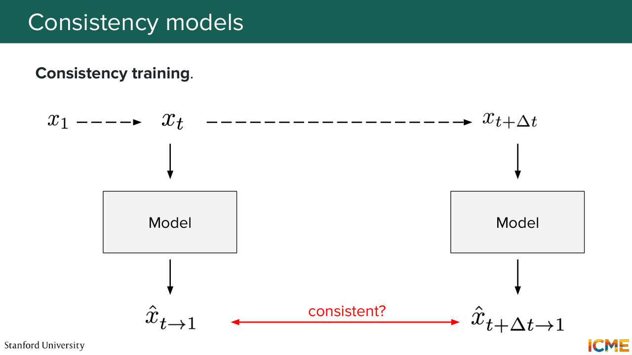
1:31:29 where you sample a clean image and then you noise it at some level t, and you noise it at level t plus delta t. And what you do is that you pass it through your model
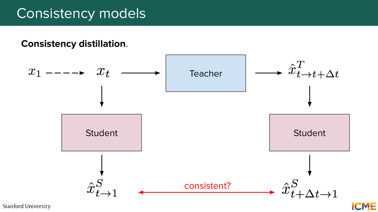
1:31:44 and try to make them match to the same value. So this is one way of doing so. There is a second way that leverages this teacher-student relationship, where denoising is not something that you would artificially do, but you would ask a teacher model to do denoising, which reflects properties that it has learned in the feature space,
1:32:09 and then you ask a student model to make predictions that are consistent to each other. So here, you might say, "OK, very well, Sherwin. But if you only force these representations to be consistent with each other, you could well have a student that says, OK, don't worry, I will always predict 0. That way, they're always consistent,
1:32:37 and maybe my loss will not be looking very pretty at the boundaries, but it's fine."
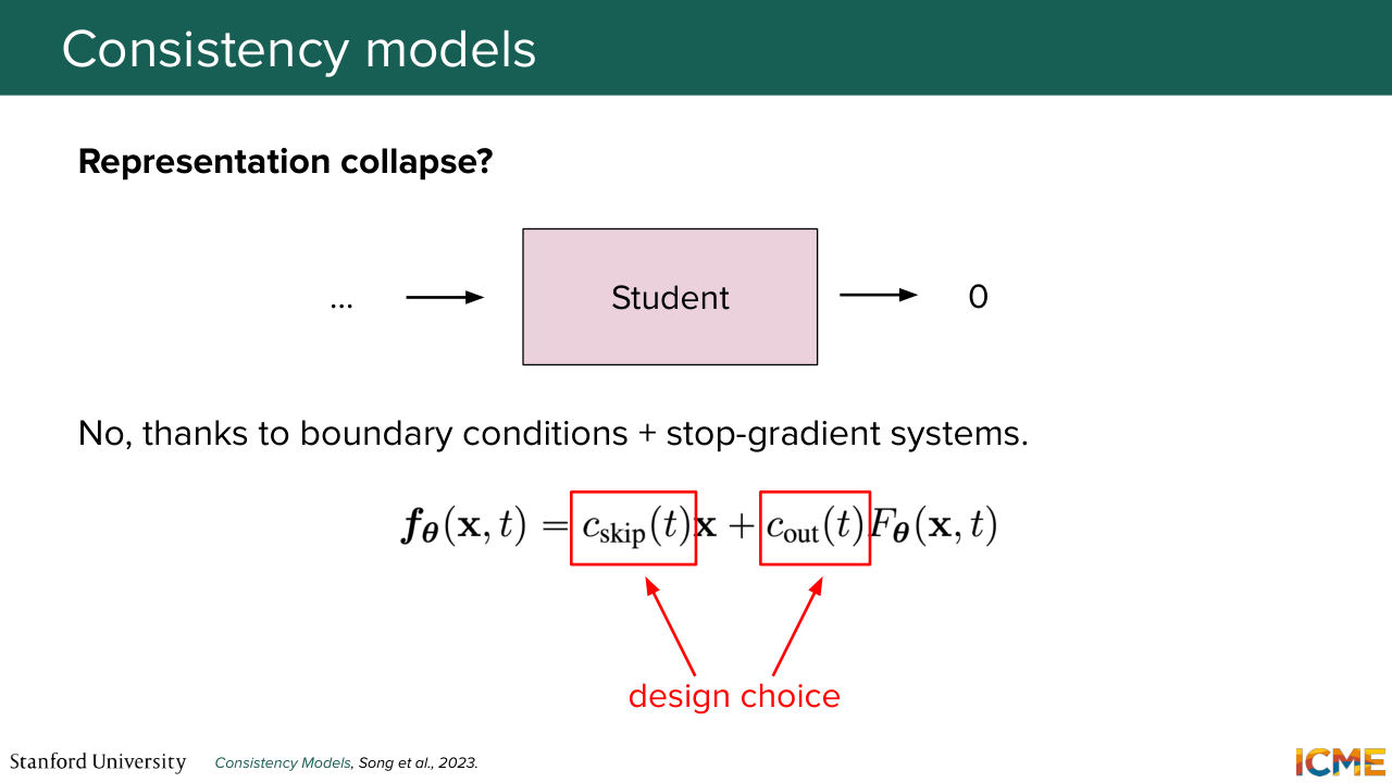
1:32:45 Well, you have a way to prevent that collapse with two tools. So one is this prediction that you get at every step, is a parameterized function of weights that we put as design. So we have it enforced. And then the second ingredient in this recipe
1:33:07 is to not backpropagate through both students, where doing so could lead to symmetrical weights updates that might not be those that actually match a fixed target. So we do that by keeping one of the students a slow-moving average and the other one actually doing the consistency prediction task.
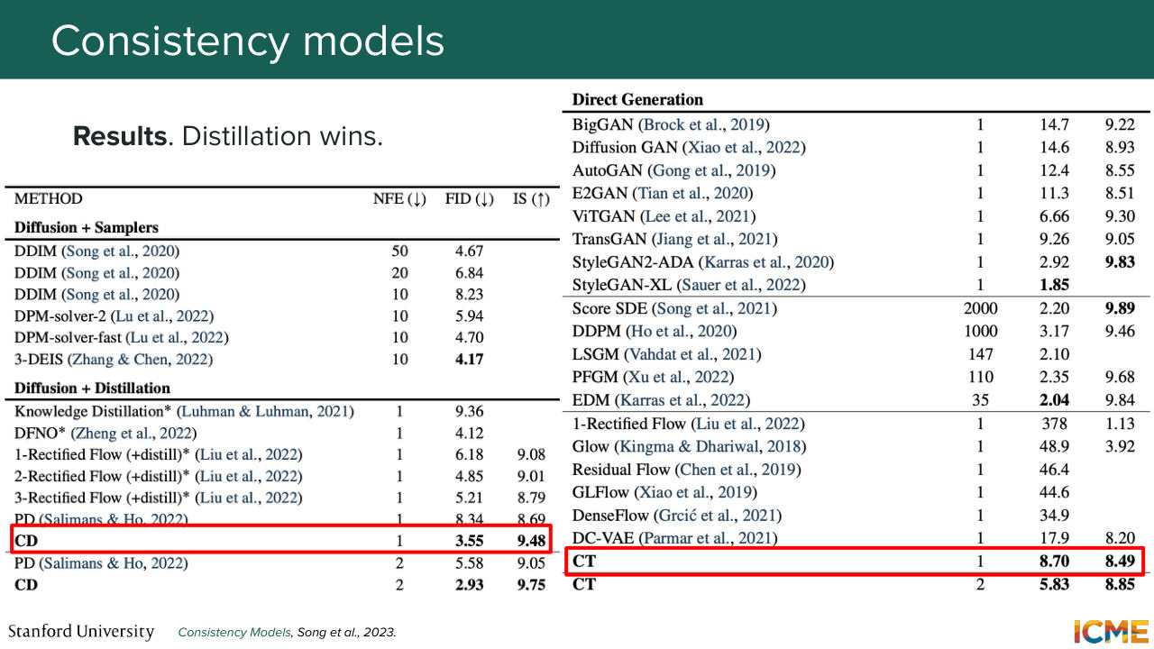
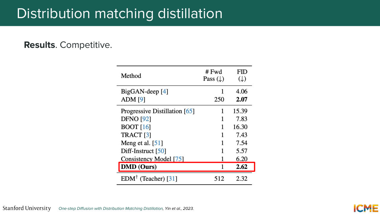
1:33:33 And when you look at what results it gets, it's quite competitive.
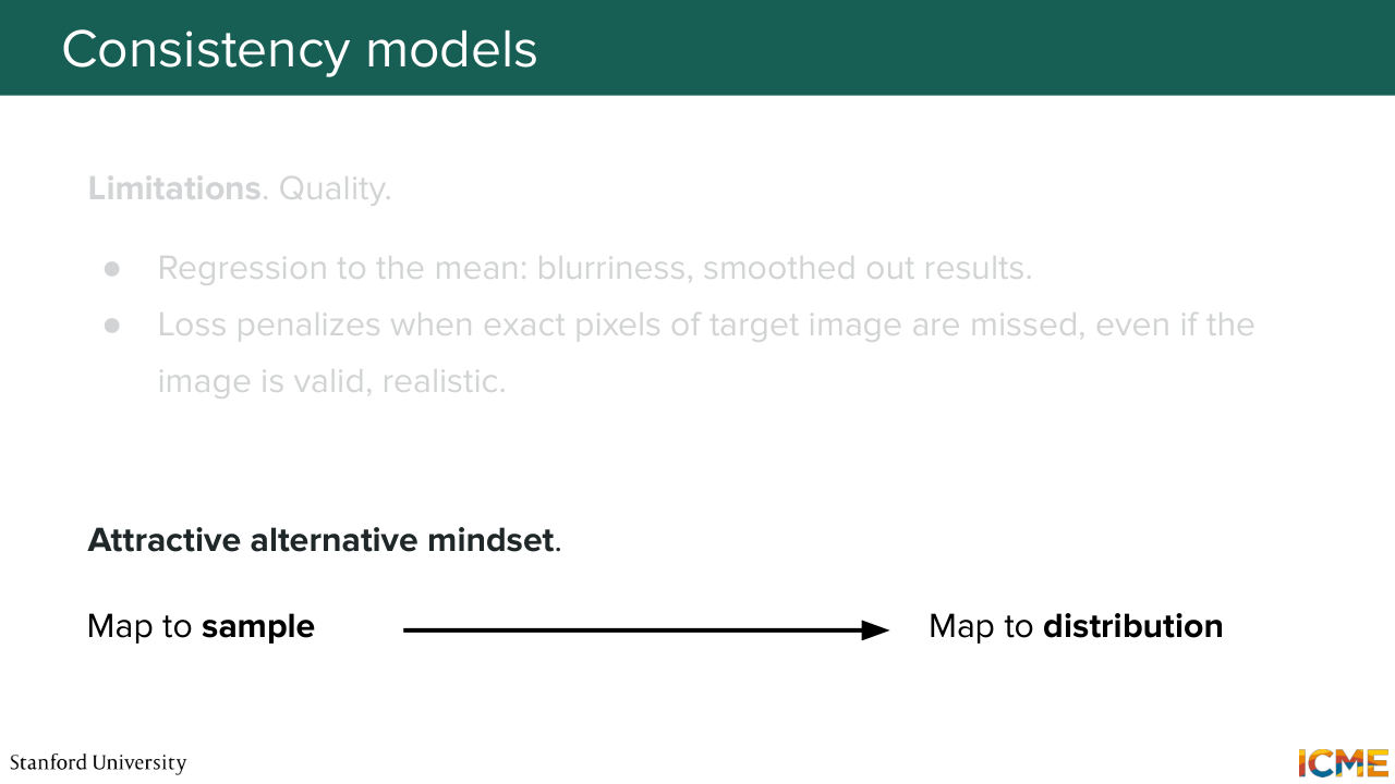
1:33:40 And you can do so in the latent space. It's called LCM. You might see in the literature. But all of these methods, what they did is that they focused on matching a given target. And one thing that you see when you have this L2-style regression loss is that you have a regression to the mean, where images don't look as crisp as you would like.
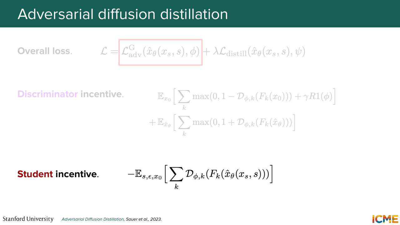
1:34:10 And GAN solves this. So let's see if there is some adversarial objective that we can introduce here to make it better.
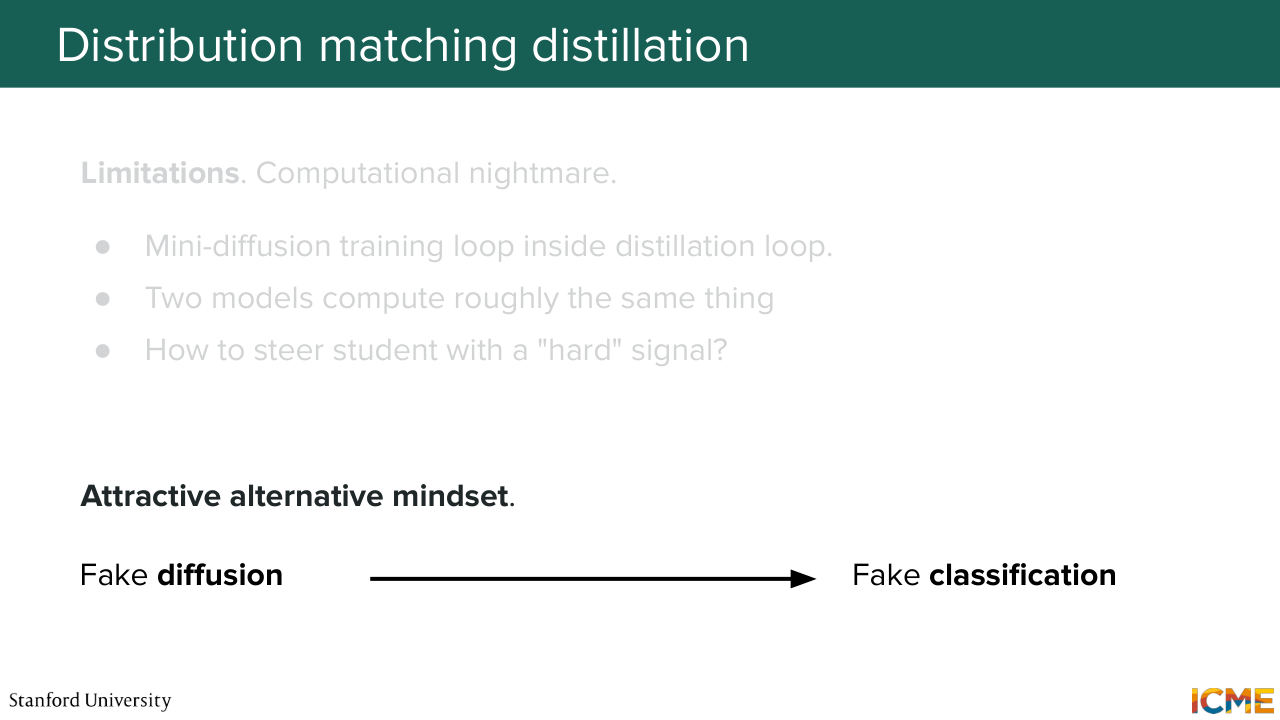
1:34:26 So before we even do that-- so we were looking at the sample level, maybe if we look at things from a distribution perspective,
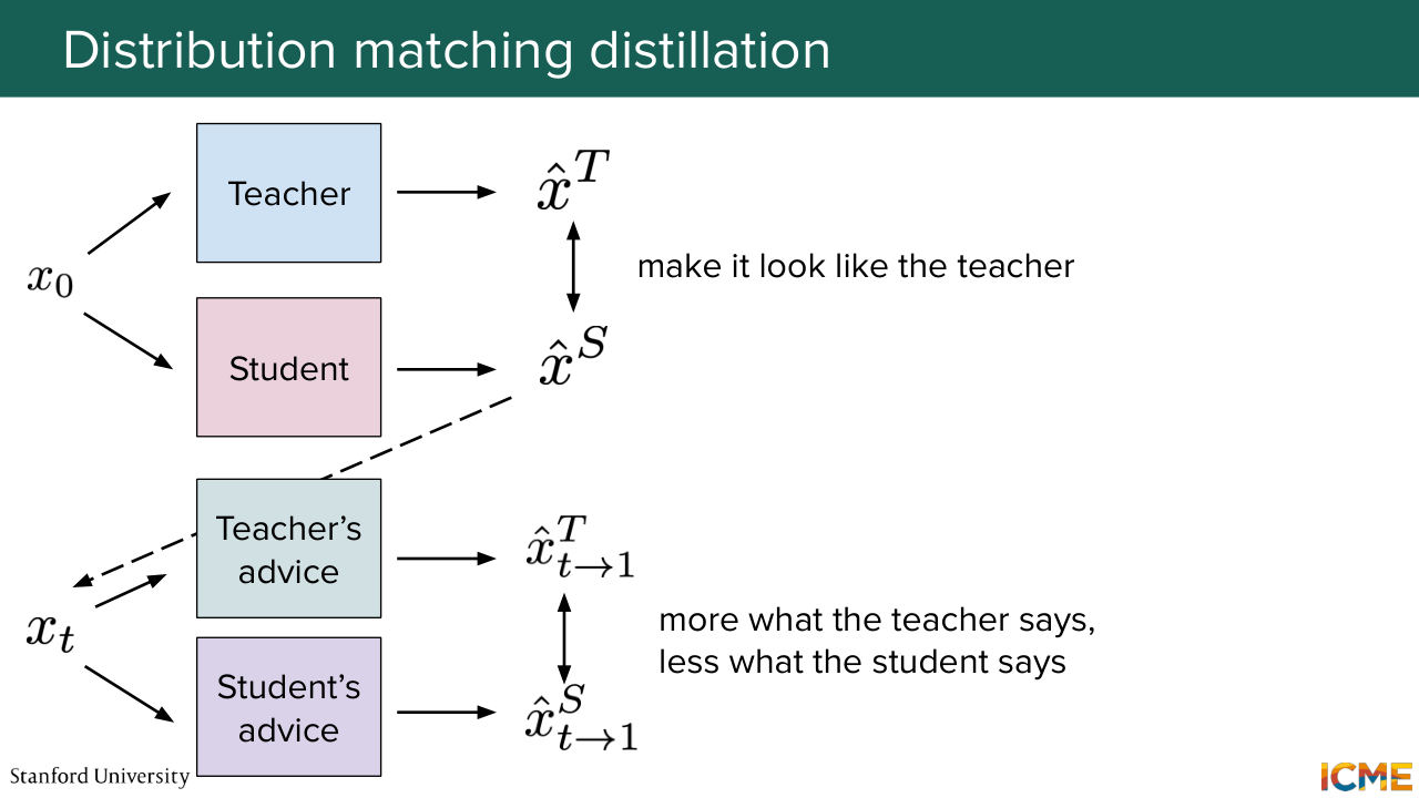
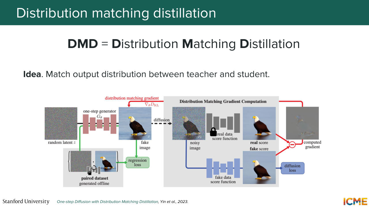
1:34:34 we could look at where we could go in the sample space that looks where we want to go rather than a straight single point. And so the mindset here is to give a piece of noise to both the teacher and student model, and then based on the student output, noise it again and ask the teacher model, and then a model that looks like the student to try to denoise it.
1:35:05 And then use their results to infer what pieces of advice the teacher and student models would give, respectively, to give the clean image, and use that signal as a way to inform what the student prediction should be. So we're going to look at this loss in details in a second. And you complement that by ensuring that the student's predictions match roughly what
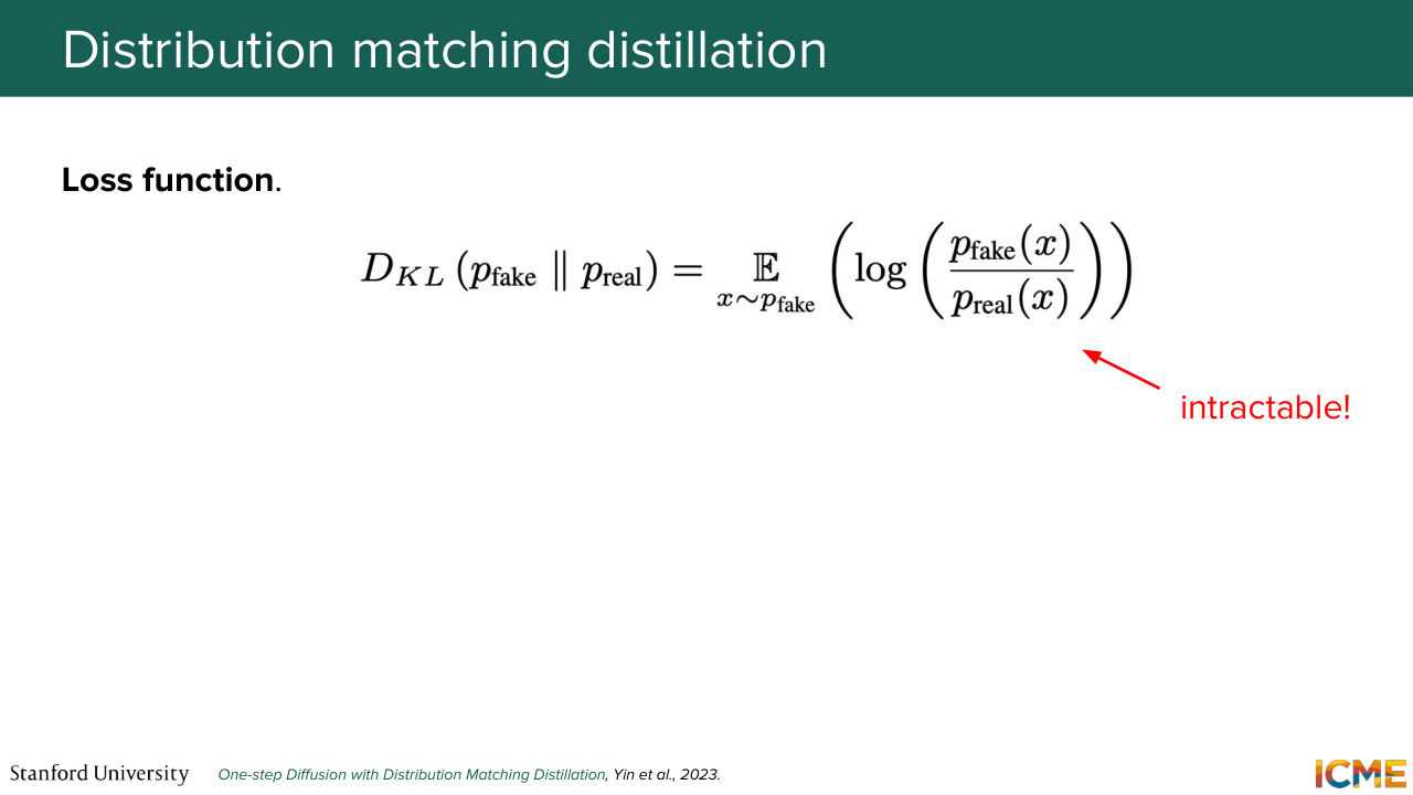
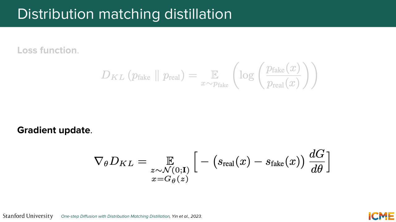
1:35:35 the teacher predictions do. And we see empirically that this helps stabilize the training. So looking at this distribution loss-- so what you're doing in practice is the KL divergence between the distribution of the fake image with respect to the real image based on a fake input. And when you take the gradient of it with respect
1:36:03 to the parameters of the student model, you get this nice interpretation of a difference of scores that you could see as a difference of velocities in the field of flow matching. And these respectively means that we want to do more of what the teacher says we should do and less of what the student says we should do.
1:36:30 And we multiply-- we do a dot product such that the parameter
1:36:36 updates reflects that goal.
1:36:42 OK, great. Yeah, I want to pause for one second just to check if that makes sense.
1:36:50 Yeah, so here-- so the question is, What's real and fake?
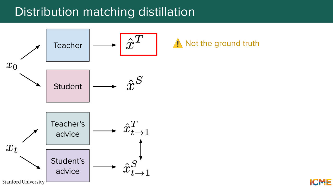
1:36:56 So here the paper uses standard denomination like used in GAN to denote respectively teacher and student. So "real" would be your true image, like what generates the true distribution that you want to reach. And then "fake" is corresponding to the distribution of the student that we want to make it as close to the real ones. So respectively, teacher and student.
1:37:25 Yeah, great point. So the question, Is there a collapse here happening? So it might. So if you were not doing that comparison between teacher and student advices, you would collapse to the mode of the teacher advice. And then the paper does some ablation study on it. And then the second piece that I mentioned earlier on, if you do not regress with the teacher's output,
1:37:52 you might see another-- not really collapse, but you would not reach the desired teacher distribution. So yeah, the answer is the collapse is bad if you were not considering this setup. But based on this setup, I think there is some hyperparameter tuning on how to balance the regression and distribution loss. Yep. Awesome. So moving on-- so I'm going to make a series of complaints
1:38:28 that are very targeted. So you're going to see where I'm going. So here we're comparing things with respect to the teacher output, which is not the ground truth. So what I've mentioned here. So I've hovered over it. But the teacher-- the student advice
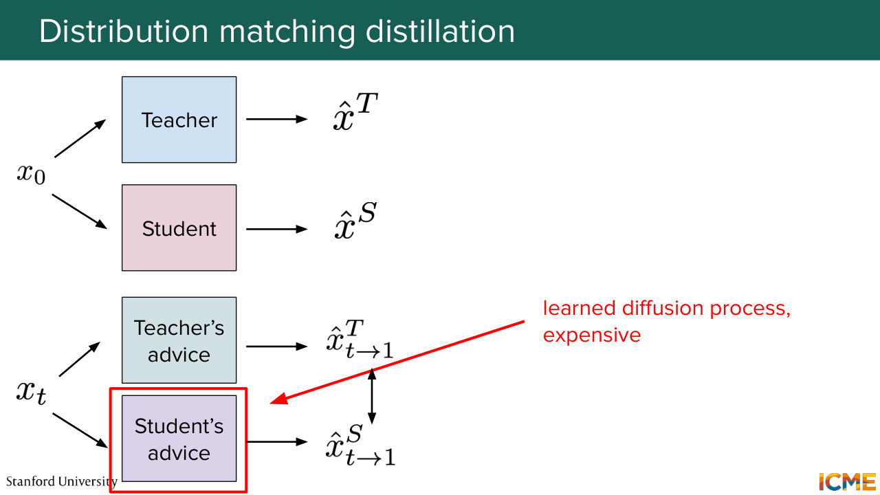
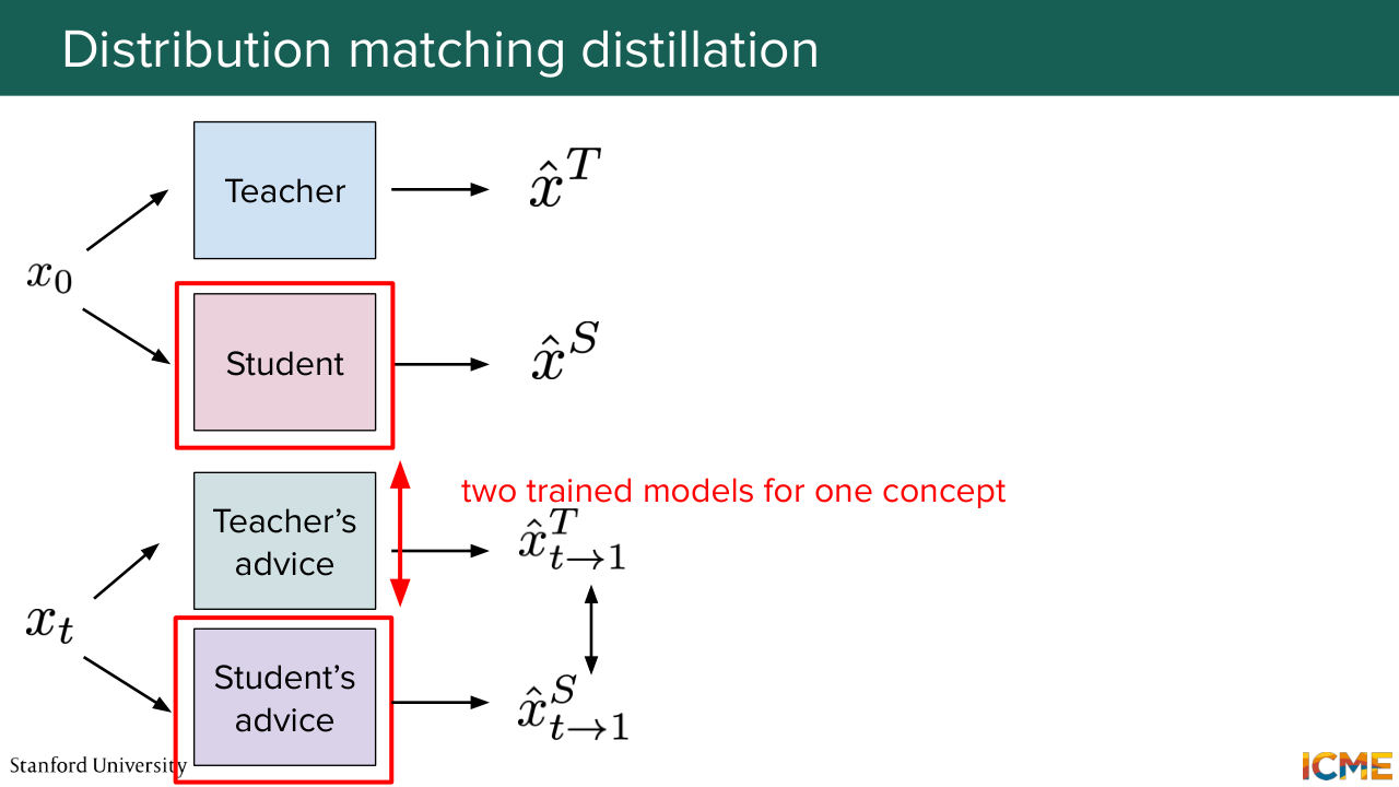
1:38:46 is actually a diffusion loop that you're running, which is quite expensive. And it's a bit of a duplicate concept with respect to the student model that you're training in the first place.
1:39:01 And this idea of providing signal with respect to teacher minus student advice might seem as a soft one.
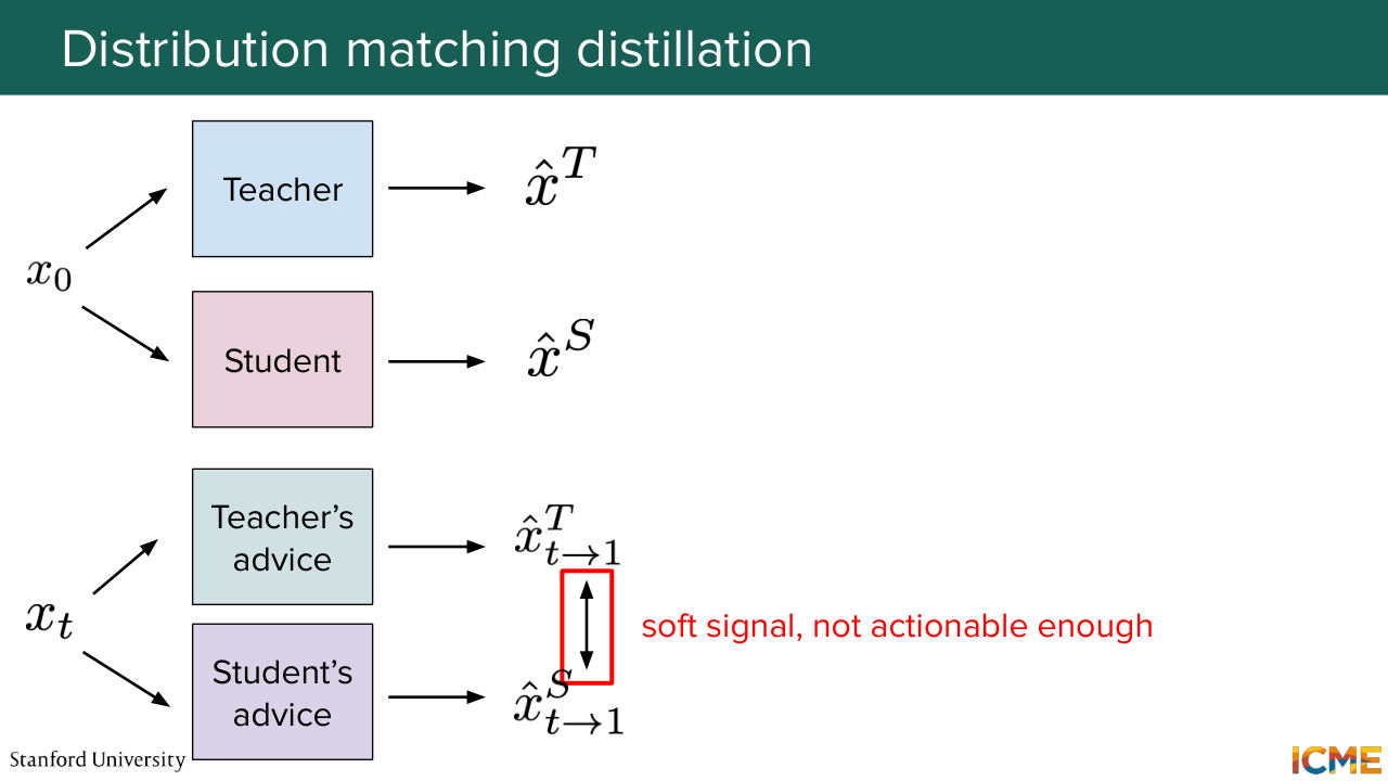
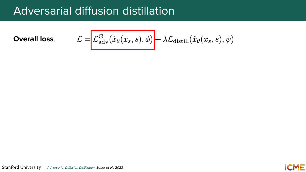
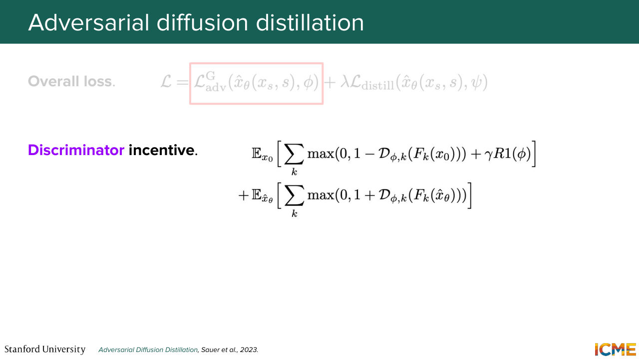
1:39:10 Is there a way to reframe it better? And yes, with GAN-like loss.
Shown briefly — discussed together with the adjacent slides.
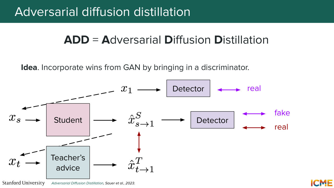
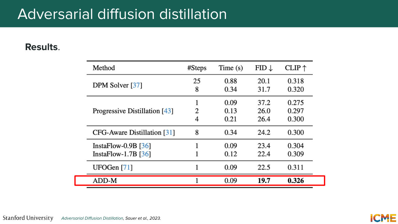
1:39:17 So this is what ADD does. And to be mindful of your time, I just
Shown briefly — discussed together with the adjacent slides.
Shown briefly — discussed together with the adjacent slides.
1:39:25 want to say the high-level is that it reframes as a classification problem that makes the problem harder in the sense that it will lead the student
Shown briefly — discussed together with the adjacent slides.
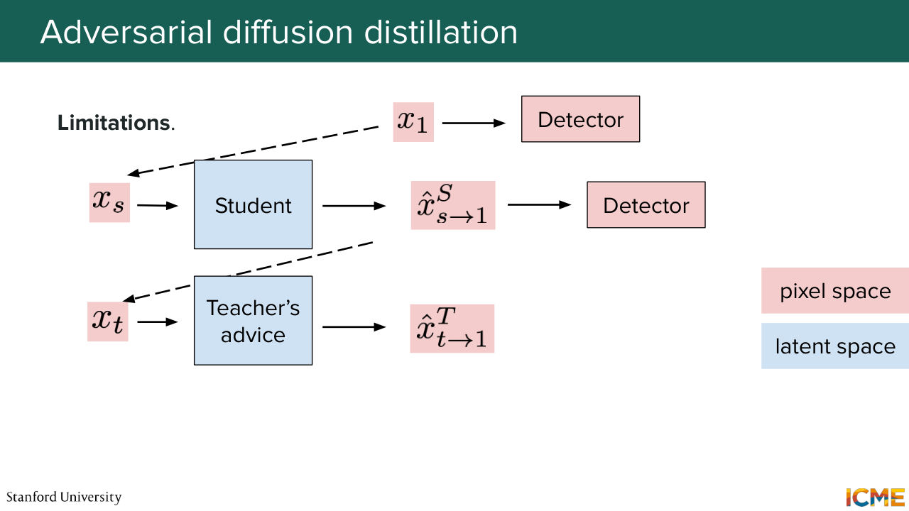
1:39:35 model to make predictions crisper. But the issue with all of this is
Shown briefly — discussed together with the adjacent slides.
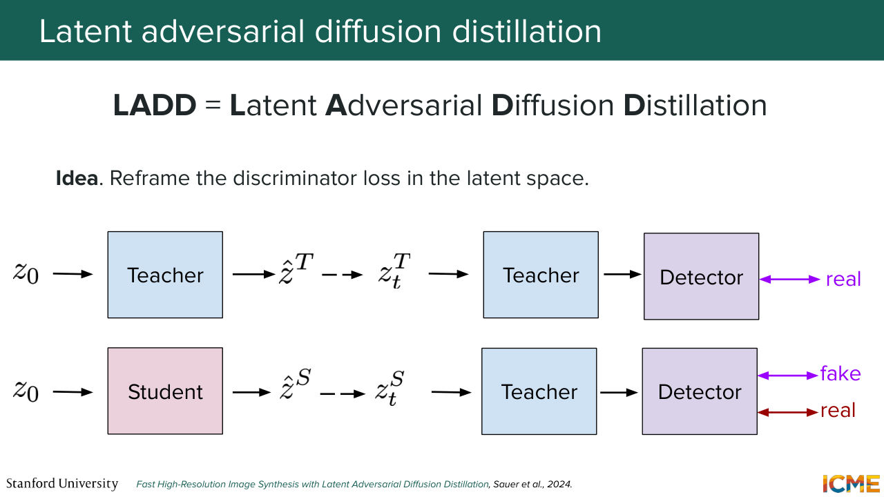
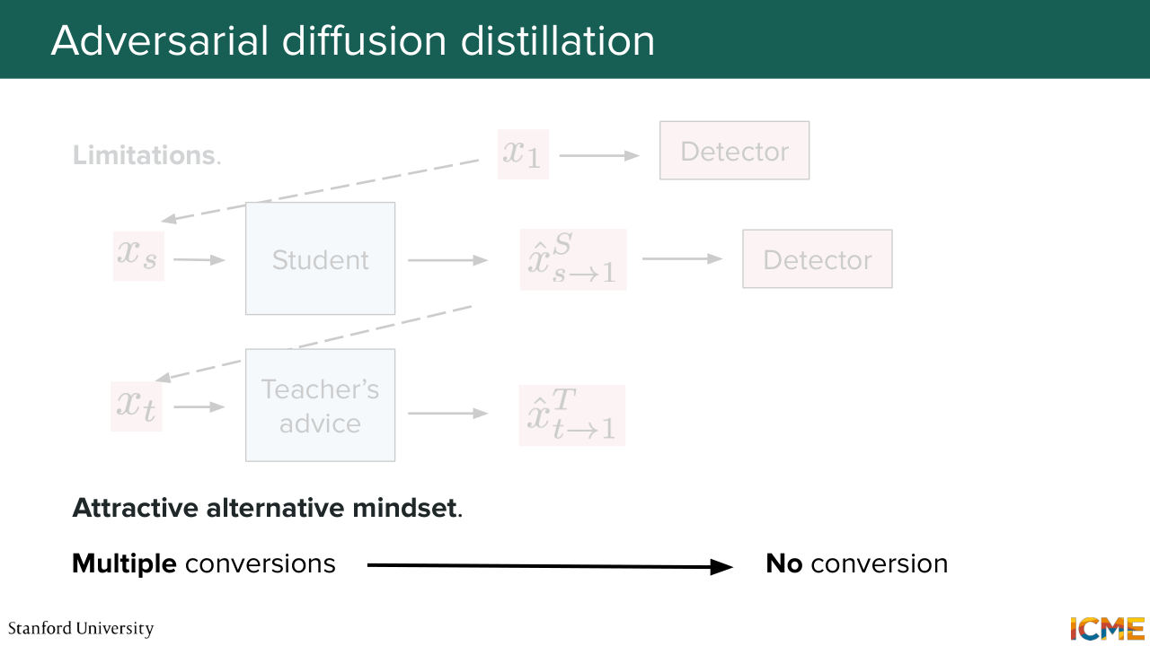
1:39:41 that you have a lot of back-and-forth going from the pixel to the latent space that later techniques, such as LADD, tries to mitigate. And this is what you're going to be used quite a bit today, so you can reformulate that only in latent space. And just to give some final words here-- so I want to say that all of these distillation
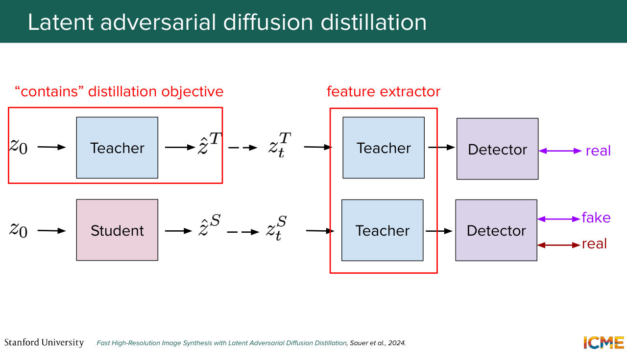
1:40:09 techniques-- they offer some kind of trade-off. For example, consistency models--
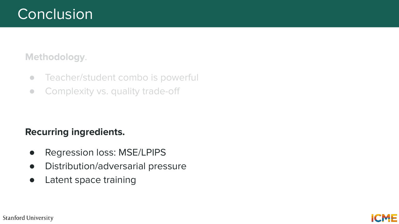
1:40:14 they might be very easily tunable with sets of LoRA weights, as Afshin mentioned, whereas, for example if you go into GAN territory, you have some dynamics in the training process that are hard to manage. And yet this duality between MSE and LPIPS loss for regression happens quite a bit, and switching the mindset to a distribution and GAN-based is great for quality.
1:40:43 And yeah. And then trends are these days to do all of this in latent space.

1:40:48 And that's all I had for you. Thanks, and have a great weekend.