0:05 Hello, everyone, and welcome to CME 296, Diffusion and Large Vision Models. My name is Afshine and I'm going to be teaching this class with Shervine who's in the back.

0:19 So before we start. I'm just going to introduce ourselves. So Shervine and I are twin brothers

0:26 and we have very similar backgrounds. So we both went to a school in France called Centrale Paris. And then we came here to the US to do grad school. So on my end, I went to MIT, and then Shervin went to the ICME Department at Stanford. And then after that, we've had pretty similar backgrounds in the industry. So we both went to Uber first, and then we went to Google,
0:57 and now we're both at Netflix. And the reason why we're so excited to be teaching this class is because back in the day, 10 years ago, when we started in the field, we actually had our first project be a computer vision project.
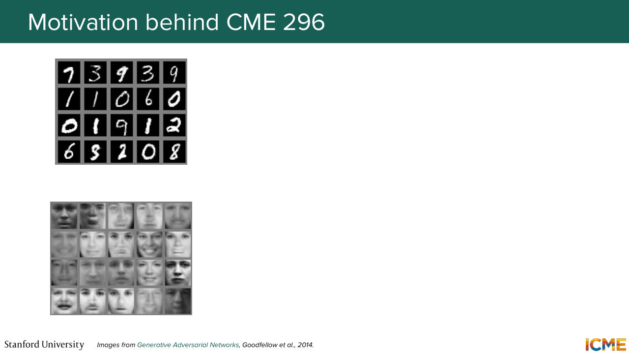
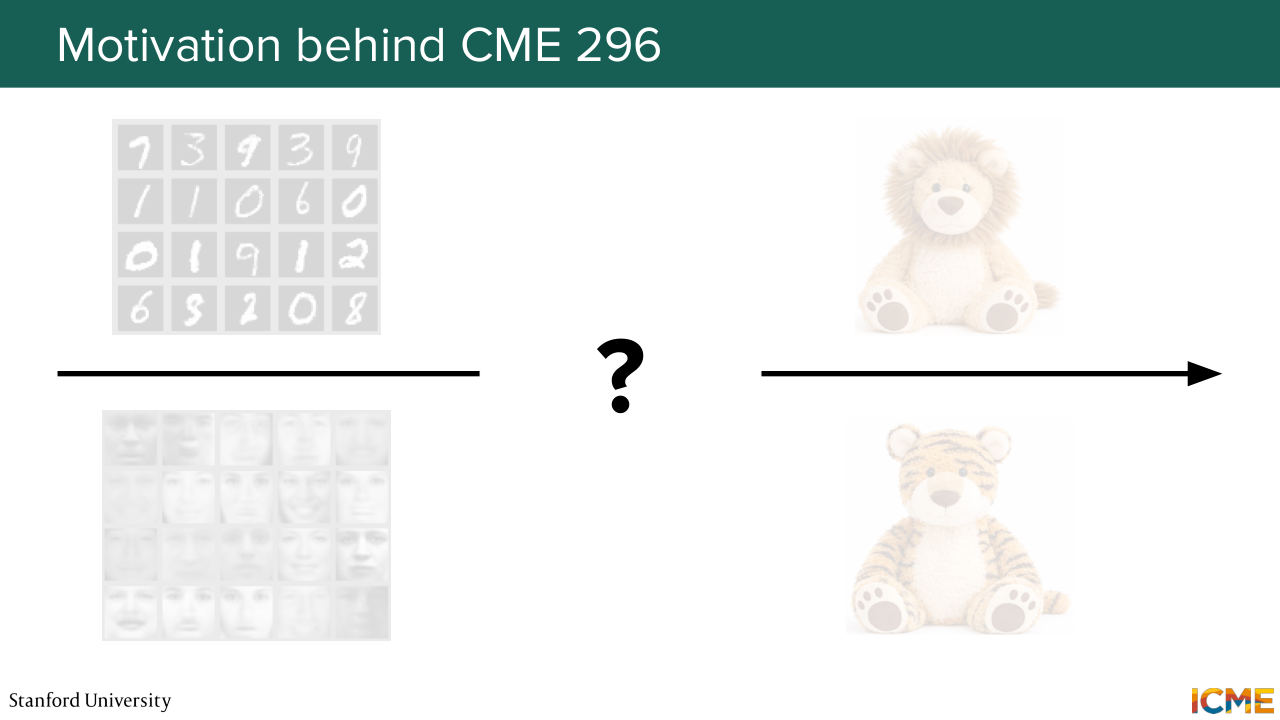
1:17 And it's been crazy the amount of progress that we've seen in the field. So this is the kind of images that we were able to generate. So it's back in 2014. So it was mostly low resolution black and white pictures. So for instance, here there some digits or human faces. And as you all know, nowadays we're
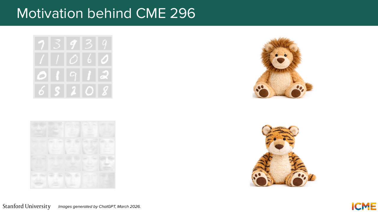
1:45 able to generate high resolution colored images.
Shown briefly — discussed together with the adjacent slides.

1:50 So for instance those ones that I generated with ChatGPT. And the goal of this class is to understand how this image generation models work and what makes them work so well. So in particular, this class has two main goals. So the first goal is to understand the paradigms
2:17 behind how we can generate these images. And the second one is to understand how the underlying models are trained and evaluated. So in case you're here in this room and still wondering if this class is good for you, I would say that this class is good if you have, in general, an interest in understanding how
2:41 image generation models work. And in particular, if this is something that you wanted to do as a career goal, if you want to go in the field of research to do peer research scientists to research how to generate images in a better way. Or if you are yourself interested, to do that on your personal time as a personal project, or just if you're here out of pure curiosity.
3:10 With that being said, I want to give a warning. So this class actually has a pretty strong set

3:19 of prerequisites, and I'm not going to hide it. So this slide is just there to enumerate the kinds of prerequisites that I think are good to have just so that you're not surprised. So first of all, in case you have some background in linear algebra, for instance, if you know what a vector is, what a matrix is, how you do operations, what is the gradient, what
3:45 is the divergence of a vector field, that would be great. If you don't everything, that's OK too. So in this class, we will not assume that you know everything,
3:59 but if you have at least some foundation, it's quite important to have it. So linear algebra is one. Second one that's quite important is probability theory. So in particular Bayes' rule, conditional marginal probabilities. What is an expectation? What is the covariance matrix, and what
4:23 is the Gaussian distribution? Again, if you don't everything it's fine, but at least most of it or at least if you've heard of it. Then you have differential equations. So here we'll see how we can use ODEs and SDEs. So ordinary differential equations
4:43 and stochastic differential equations and how they matter, and how we solve them. And then last but not least, there's some basics of ML. So if you know how you train a model, just in general using a neural network, how you do training, how you do inference, that would be great. But again, we will try to review these concepts
5:09 in a non-exhaustive way in an intuitive way. But yeah, just knowing those, I think, would be great. So that's one Warning. The second thing that I will say is that this field
5:23 is very technical in general. So if you read a computer vision image generation paper, you will see that there are formulas all over the place. So the goal of this class will not be to go into all of these details. So we will try to strike a balance between not shying away from the math, just understanding what are the important formulas, but also at the same time,
5:50 just understand why they're there. So we'll try to make a big emphasis on intuition. All good so far? OK, great. So just moving on to some logistics.
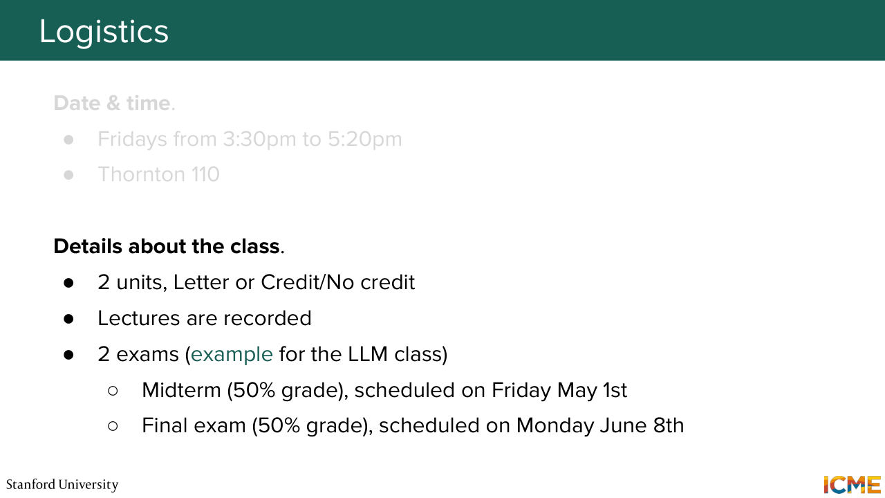
6:08 So we'll have this class every Friday from 3:30 to 5:20 in this class. And just again logistics. So it's a two unit class. You can take it either as a letter or credit non-credit. So as you can see with the setup, the lectures are recorded. We'll try to post the videos by Saturday evening.
6:34 So for you watching remotely, if you don't come to class, it's all good. We'll be just publishing the videos within a day of it happening. And then in terms of the exams. This class has no homework, but we have two exams. One is the midterm and the other one is the final. And here, it's the kind of exam that you may or may not like,
7:03 but it is a pen and paper kind of exam. Meaning the lectures that we will do will be about concepts that will be covered in the exam. And the important thing is to not know all the details, again, just the general formulas and mainly the intuition
7:29 as to why they're there. So in case, it's a little bit vague for you, we have a similar class that we do for LLMs. I'm not sure if you've heard CME 295. So the format of the exams is very similar. So in case you're interested, we put just a link to one kind of exam that you can expect. Of course, it will not be the same questions because it's also different topics, but it will give you a good idea.
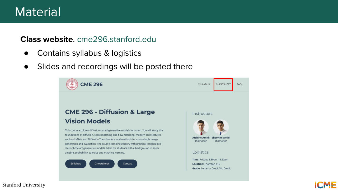
8:04 Any questions on the exams? Super clear? Yeah I know it's the first lecture, and I'm talking about exams already. So yeah, don't worry. It's four weeks away and we have time. And yeah, it's a fun class, I promise. Cool. In terms of the material, we have a class website,
8:31 and on that website we'll be publishing the slides and the recordings as well. So just so that you have a way to get the slides in advance for annotation purposes, one thing we will do is to publish the slides the day before the lecture, so Thursday evening. So you can get the slides and make some annotations. And if you saw, there is a tab also top right cheat sheets.
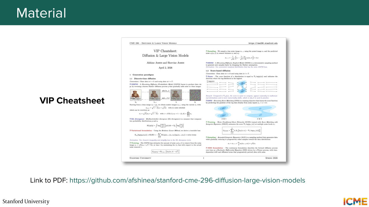
9:02 We also published a condensed four page cheat sheet on the content of this class. So it gathers all the main formulas and concepts. So our goal is-- if you look at it today, if you don't understand parts of it, our goal is by the end of this class to have everything be very clear.
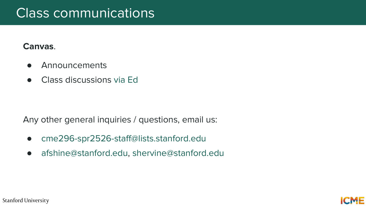
9:30 So if we achieve that goal, I think that's great. Cool. OK. So last thing. So for any announcements, we'll be posting them on Canvas. And then we have a forum for class discussions on Ed. And of course, feel free to reach out to us. So there is the addresses here on the slides,
9:53 if you need anything. Cool. I think these are all the logistics. Is there any questions so far on just how the class works? Yeah. So the question-- so I'm going to also repeat the question for people at home. So how long is the midterm and the exam? It's one hour and 30 minutes.
10:24 OK, cool. I think we're all good then. Great. So let's get started. So I just want to call out that in the slides of this class what we will do is to explain the concepts in the main part, but we will always put a reference to the paper that talks more in depth about what we're talking about, just because we only have, I believe,
10:52 eight lectures of two hours, so we have nowhere near covering everything in detail. So yeah, feel free to look at them. They will not be required to know for the exam, it's just for your own reference. OK, an important note. So I mentioned that the papers in the field are crazy in terms of technicality and math formulas,
11:18 the same goes for conventions. So you will see that from paper to paper, things are noted differently, and it can be very confusing. So for instance, you will see there is a time t that sometimes is between 0 and 1, sometimes it's between 0 and T, sometimes it's in reverse, sometimes a epsilon is not a Z or X0 or X1, et cetera.
Shown briefly — discussed together with the adjacent slides.
Shown briefly — discussed together with the adjacent slides.
Shown briefly — discussed together with the adjacent slides.
Shown briefly — discussed together with the adjacent slides.
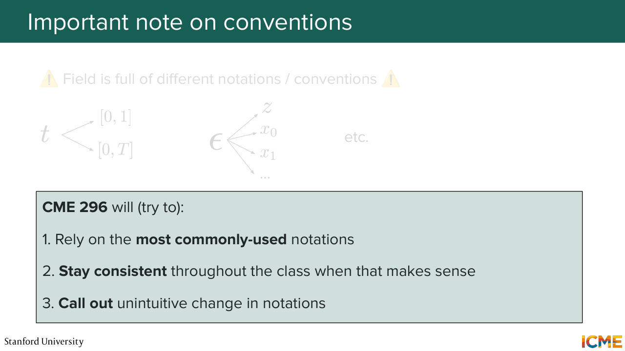
11:47 So in this class, what we will try to do is three things. First is we will always try to rely on the most commonly used notations, so that when you go and refer to those papers, you're not lost. The second one is we will try to stay consistent as much as possible. So if we take a notation, we'll try to keep it so that you're not confused.
12:15 And if we don't keep it, we'll just make sure to call it out.
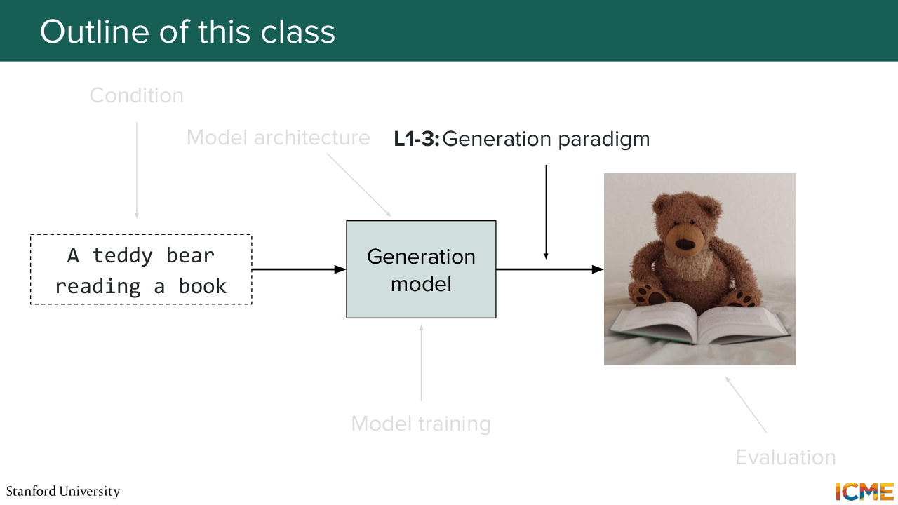
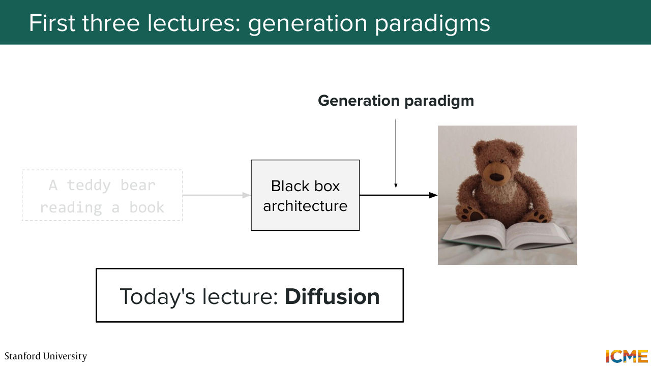
12:23 OK. Great. So as I mentioned this class is all about understanding how image generation models work. So here you have a typical setup where you have let's say a prompt where you specify what you want to generate. So here I want to generate a Teddy bear reading a book. And I put that in some model.
12:49 And then the model generates an image. So this is what we want to cover. But as easy as it seems, it's actually quite complex. There's a lot of things moving pieces everywhere. And I'm going to call out the main moving pieces that we'll cover. So the first one is if you suppose
13:15 that you have some model, how do you go about generating images? What is the process of generating images? So in the text world is quite easy. The most common paradigm is you generate one token at a time, because that's also what people talk and how people write, so it's quite intuitive, but in the image world, it's not straightforward.
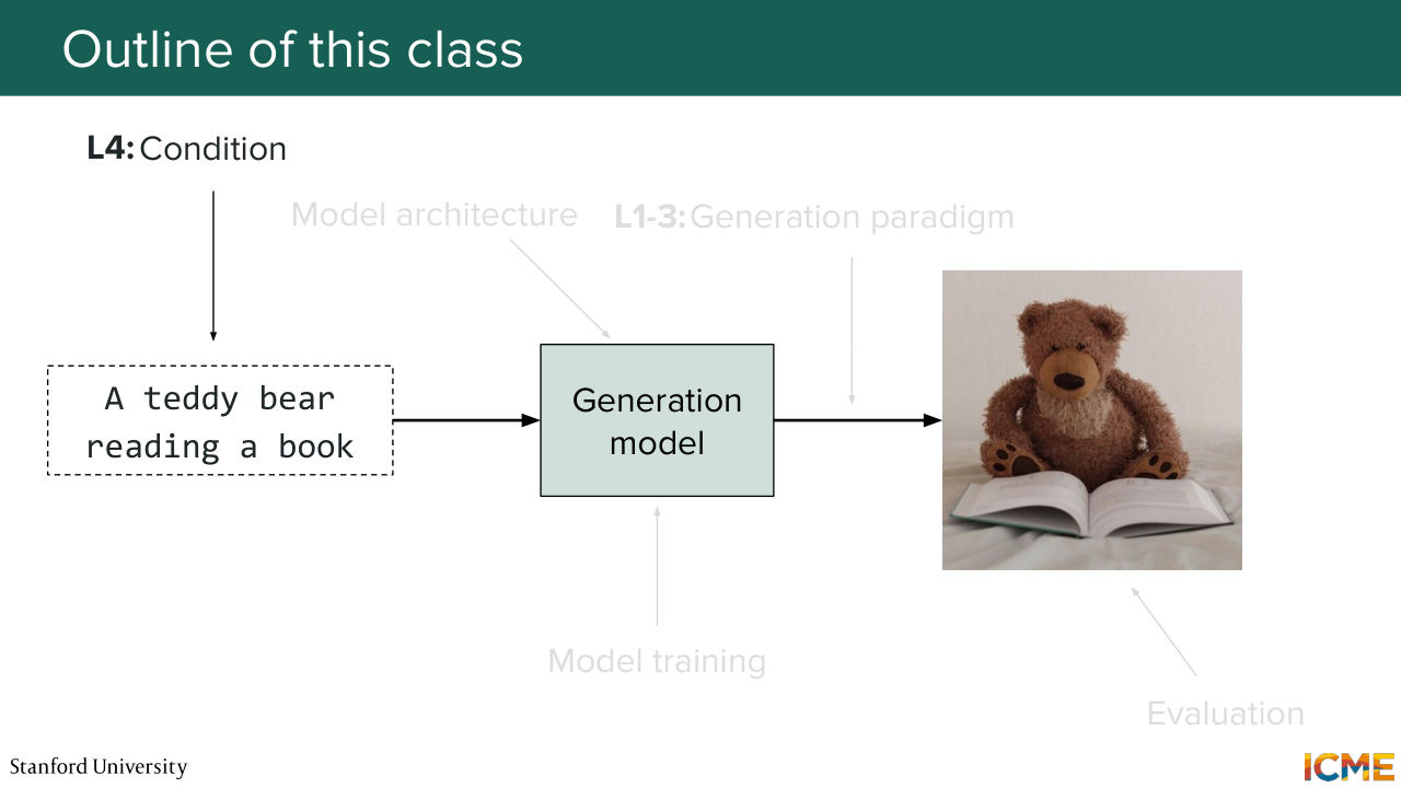
13:43 So we will focus lectures 1, 2, and 3 on this part. And we will cover the main ways of doing it, which are the most commonly used today, which are diffusion, score matching, and flow matching. Then we will look at how we can condition our model to generate
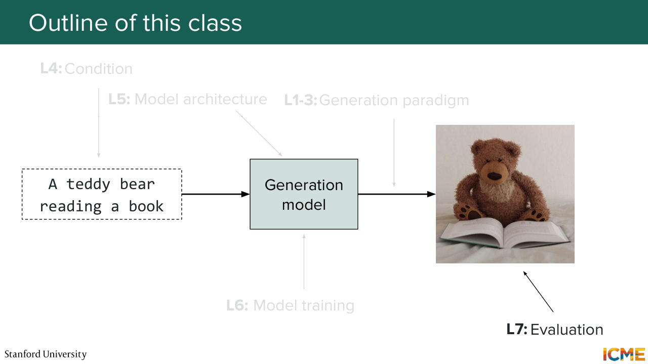
14:11 these images to start with. So we'll cover that in lecture 4. So in some sense we want to guide the model to generate something, and this is what we will cover. We'll also cover how to represent images in a space that quote unquote, "makes sense." So lecture 5 is going to be about the model architecture.
14:39 So we'll take a look at the backbones that are most commonly used today. So back in the day you may have heard of u-net as being something that was used. But there's currently a convergence of architectures more towards transformer based architectures, such as the diffusion transformer and variants such as the multimodal diffusion
15:02 transformer, and we will take a look at those there. Then lecture 6 will be around knowing how to train those models. So in particular, how do you have your model understand how to generate images and any post-training approaches that you may also need. There's also something that is quite important, especially
15:28 in the industry, which is you have your model, but you want to run it quicker because you have some constraints in your setup so we will see also distillation techniques. So this will be in lecture 6. And finally lecture 7 will be about evaluating images. Because if you look at an image-- I'm not sure about you, but it's not super obvious
15:56 how you would define an image as being great or not great. So you will see that the field is full of acronyms when it comes to metrics. And each of those is there actually for a reason and we'll try to see that. And then the second thing that we will see is this emergence of multi-modal LLMs
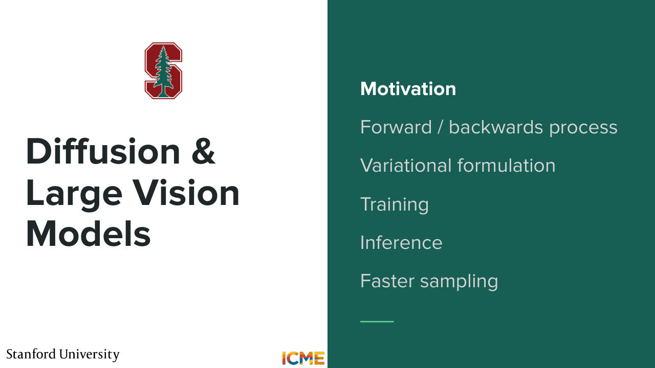
16:23 that also understand images that can also help us to evaluate them. So this will be for lecture 7. And today as mentioned, we will start with the generation paradigm one. And in particular, we will look at diffusion. So who has heard of diffusion. Yeah, OK so everyone.
16:51 So we will see beyond the general intuition of roughly how that works. We'll see exactly how this was defined and what is making this objective be tractable in practice. So one thing that I want to call out is in the first three lectures, we will assume that there is nothing as input.
17:20 So we have some distribution of data that we use as training sets. And what we want is to generate images that are like them. So in mathematical terms, we want to have a model that is able to sample an observation from the data distribution.
17:38 So in a sense we'll only focus on unconditioned generations
17:43 for the first three lectures including this one.
17:49 Cool. So speaking of data distribution. So let's suppose we have a set of images.
Shown briefly — discussed together with the adjacent slides.
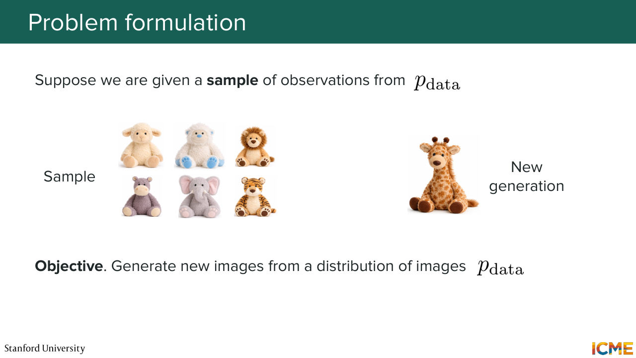
17:57 So here a long running example will be Teddy Bears. So here let's say we have a collection of Teddy Bears as training images. Our goal is to understand a way to sample an observation from that data distribution that is new. So what we want to do is to be able to generate an image that
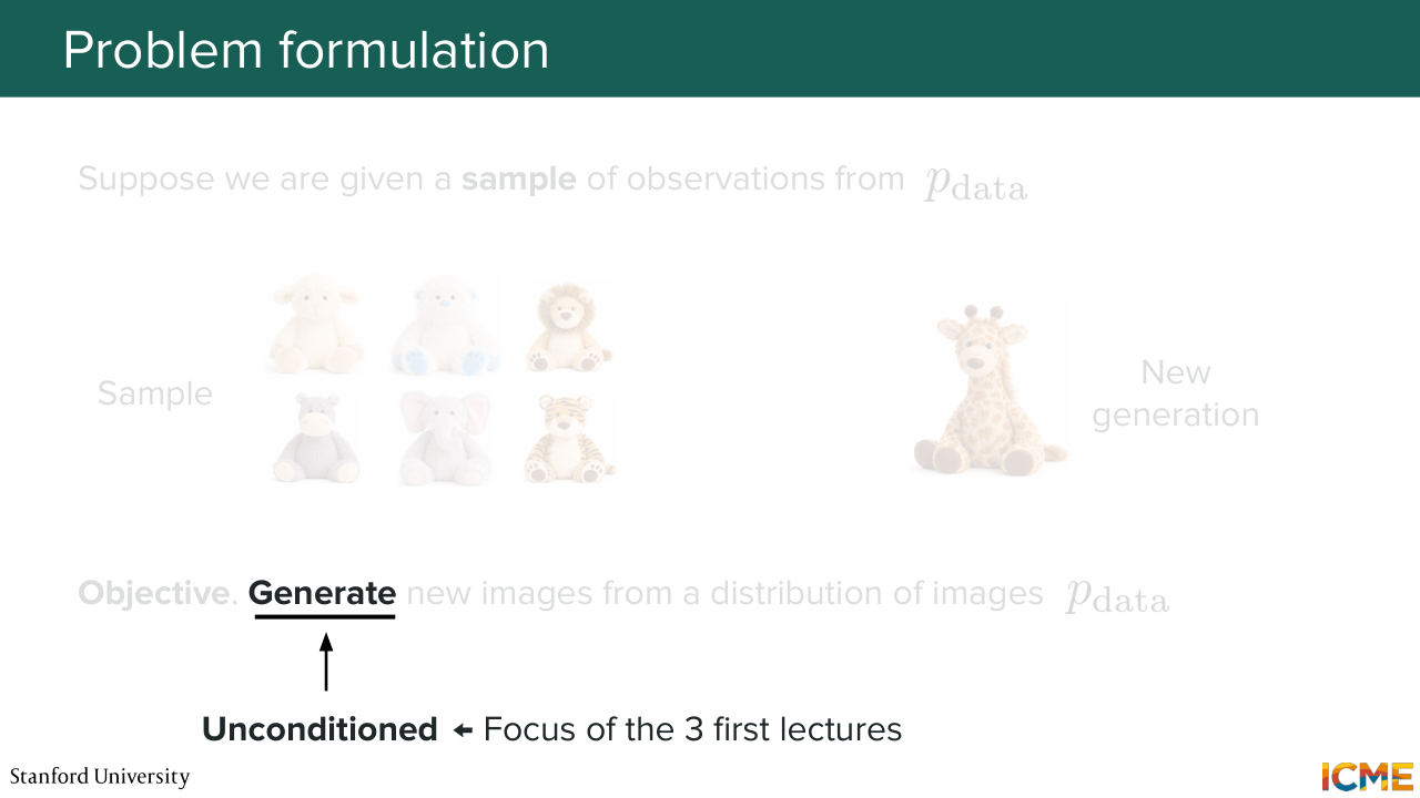
18:22 is in that data distribution. So here for instance giraffe. And again, just emphasizing that this is unconditioned. We're not putting anything as input. We just want to generate a sample that is following that distribution.
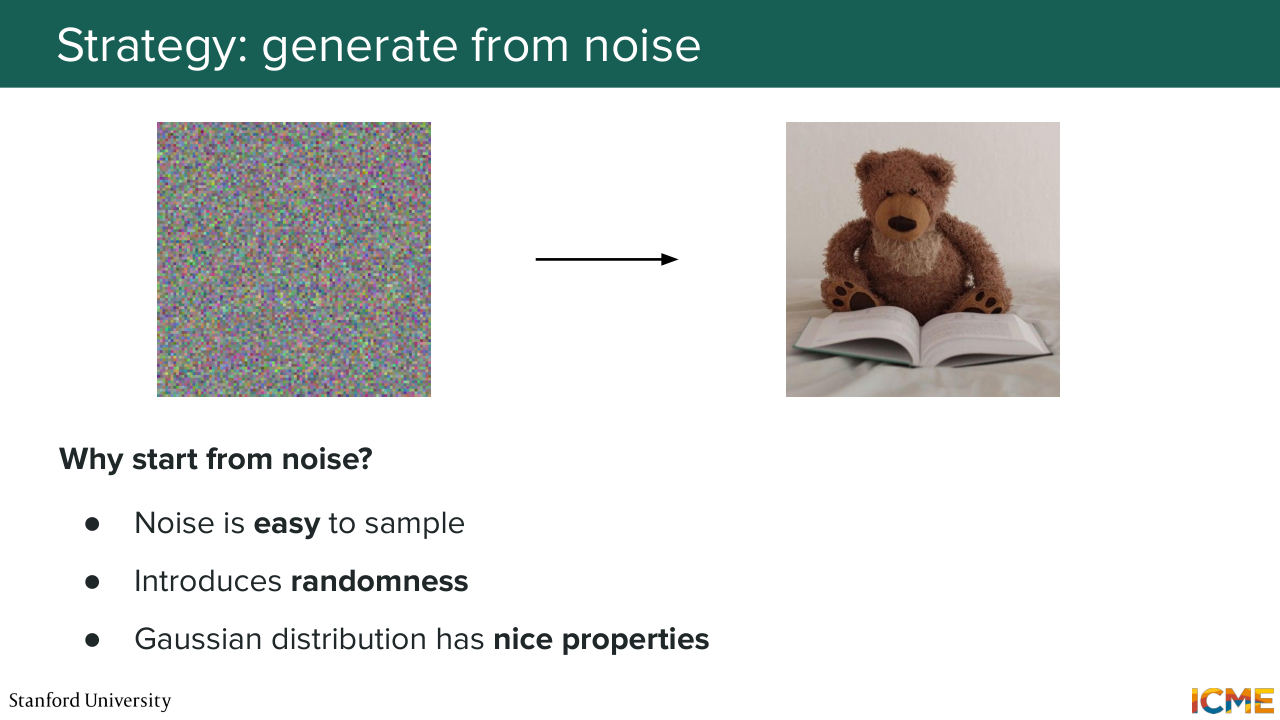
18:42 So how do we do this? So you will see that most if not all methods out there, they all have something in common. They all start their image generation process from noise. So they start from noise, and then they refine the image to be the final image. So I want to just spend some time on why that is the case.
19:10 So we'll define what noise means, by the way because you will see the term noise and then you will see this grayish image. So you will see that this noise is actually something that you can sample from an easy distribution, the Gaussian distribution, spoiler alert. So the first reason why it is something that we want to do is because it is easy to sample from noise.
19:36 It is easy to have some noise. The second thing is noise has some randomness that allows you to generate different images. So even if let's say you have a condition, if you start from noise that is different, let's say from another generation, you will be able to end up with a different end image just because the starting point is different.
20:05 So the second reason it introduces some randomness. And then the third one is, as I mentioned, noise is basically equal to a Gaussian distribution, and that distribution just happens to have very nice properties. So it simplifies a lot of the math and we will see a little bit how that is the case in the diffusion case.
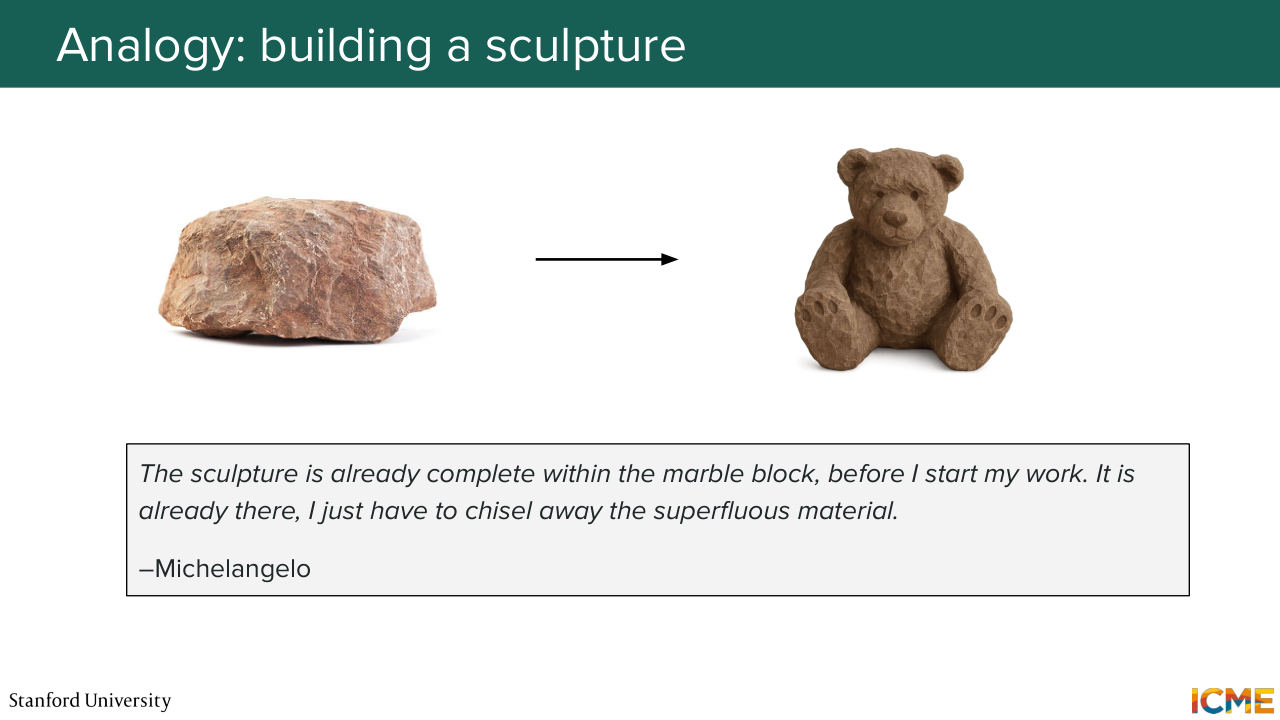
20:34 Cool. So intuitively does that make sense, that noise is a good starting point? Yeah? OK, cool. And just to complete that intuition, in the 3D world, how sculptors go about sculpting their sculptors, they start with some rock. And you can think of this rock as having shapes
21:01 that are a little bit noisy. It's not something that you are defining. It's something that is just there. And that will be different from a rock to another. So one analogy that I like to think of is this image generation process is a little bit if you were a sculptor and you wanted to sculpture from rock. So yeah, I will leave you with that quote from Michelangelo that I think also reflects that pretty well.
21:30 Cool. Yeah. So when you say uniforms, you mean the same thing? Like let's say blank? Yeah so the question is, why do you want to start from noise, but not from something that is predefined, let's say a black-- sorry a white canvas, let's say. So yeah, great question. So you will see that what makes the end--
22:21 so the generation process sometimes involves some randomness in the generation process, sometimes it does not. The randomness is something that occurs at the starting points. So if you were to always start your process from the same starting point, given that everything else does not introduce some amount of randomness, you will always end up at the same endpoint.
22:53 So in a sense, what you want is to have some variation introduced somewhere in order to not always end up at the same place. So I'll give you an example. This Teddy bear reading a book. If you use a generation paradigm that does not have any stochasticity in its process, then if you always start from the same point, then you will always end up at the same endpoint,
23:20 and that's probably not something that you want just for diversity purposes. So that's the intuition. Yeah, great question. Cool.
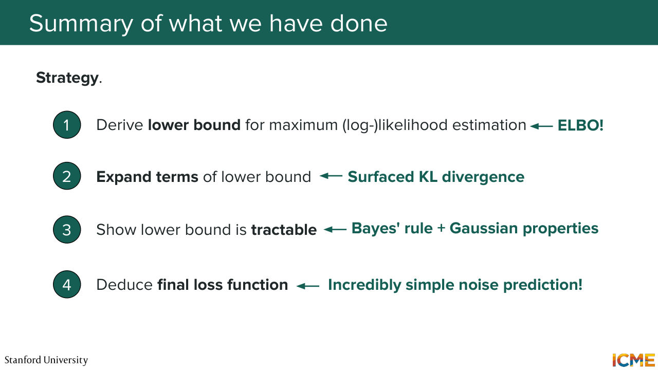
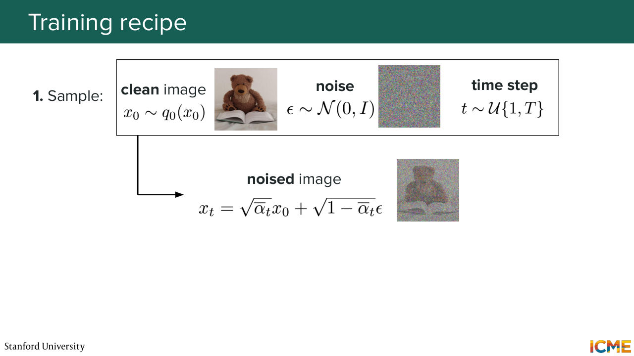
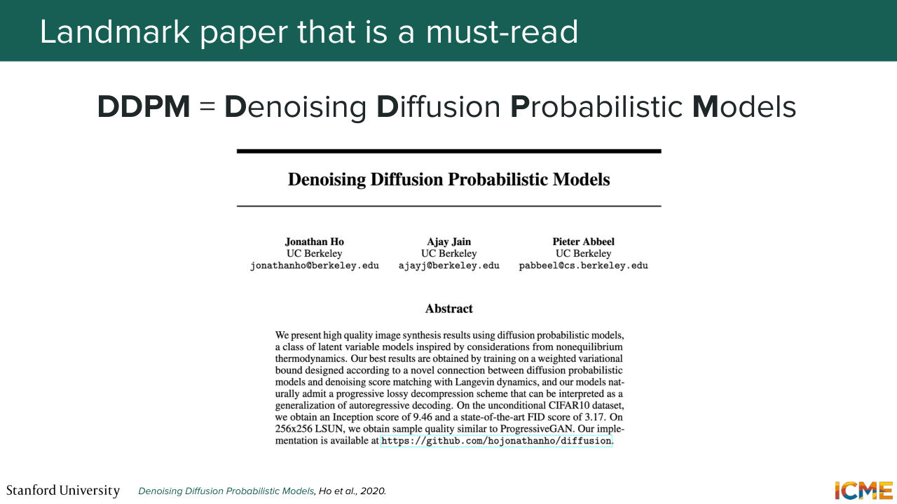
23:34 OK. So what we'll focus on for this lecture is a landmark paper that I will talk a lot in depth, that's called DPM. That was the first that applying this diffusion paradigm for images in a successful way. So what we're going to do is to go
23:59 through what makes this approach work so well, and the underlying mechanisms that lead to the loss function that we have. So in particular, the idea that we have here is what we want is to generate new images. So what we do have is a set of training images
24:26 and our goal is if we were to start from noise, how would we be able to recover those images? That's what we want to learn. Because as I mentioned during our generation process, our strategy is to start from noise and end up with a clean image. So here what we want to do is to use those training set images
Shown briefly — discussed together with the adjacent slides.
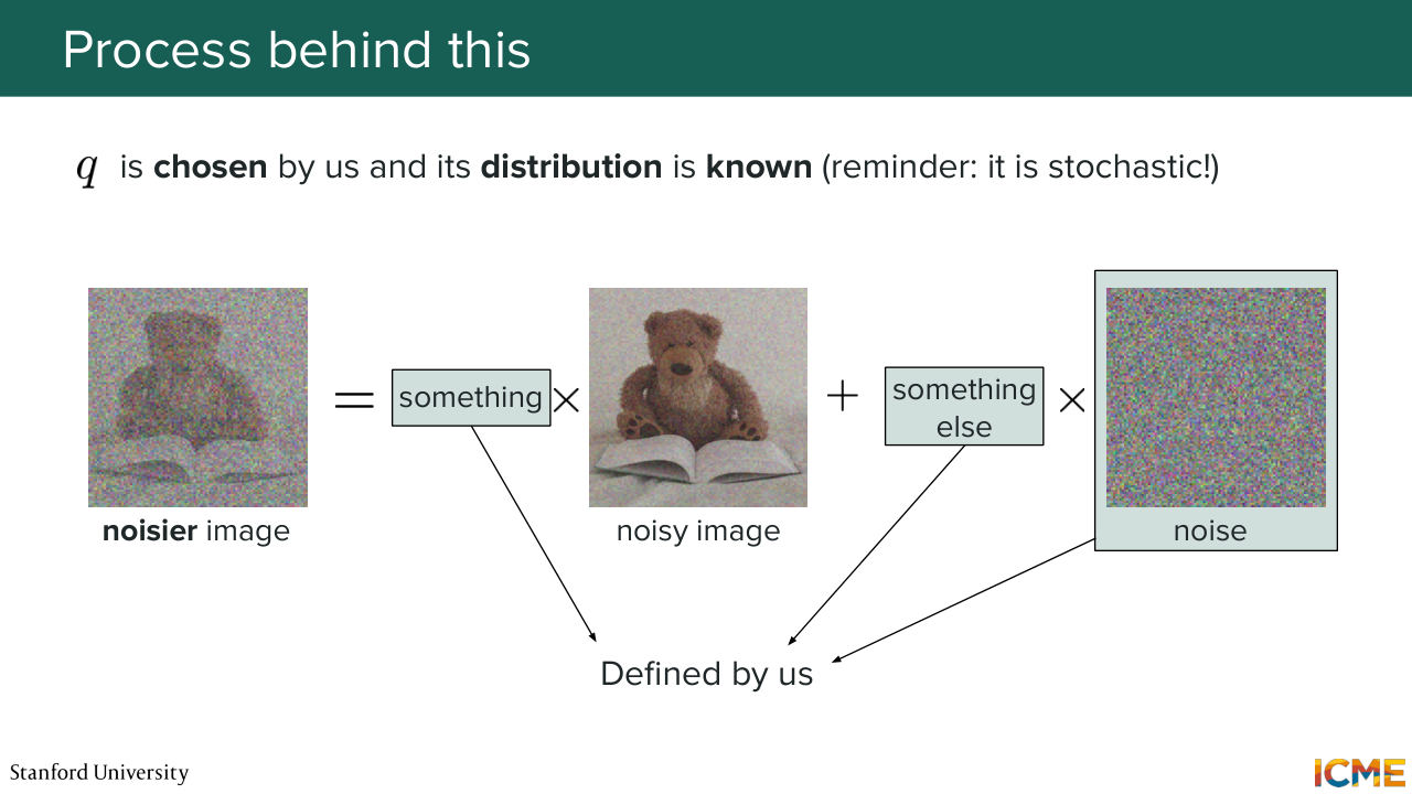
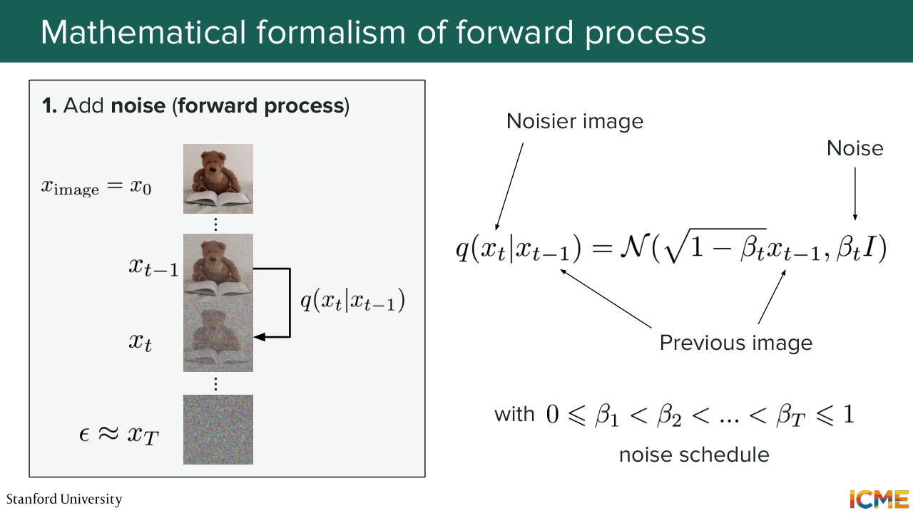
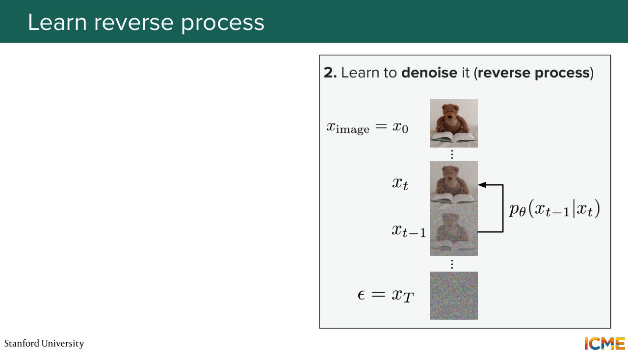
24:53 to learn that denoising process. So in that regard, we have two processes that have a very particular name. So the first one is called the forward process that amounts to taking an image from your training set, and you are actually corrupting that image. You're adding some noise.
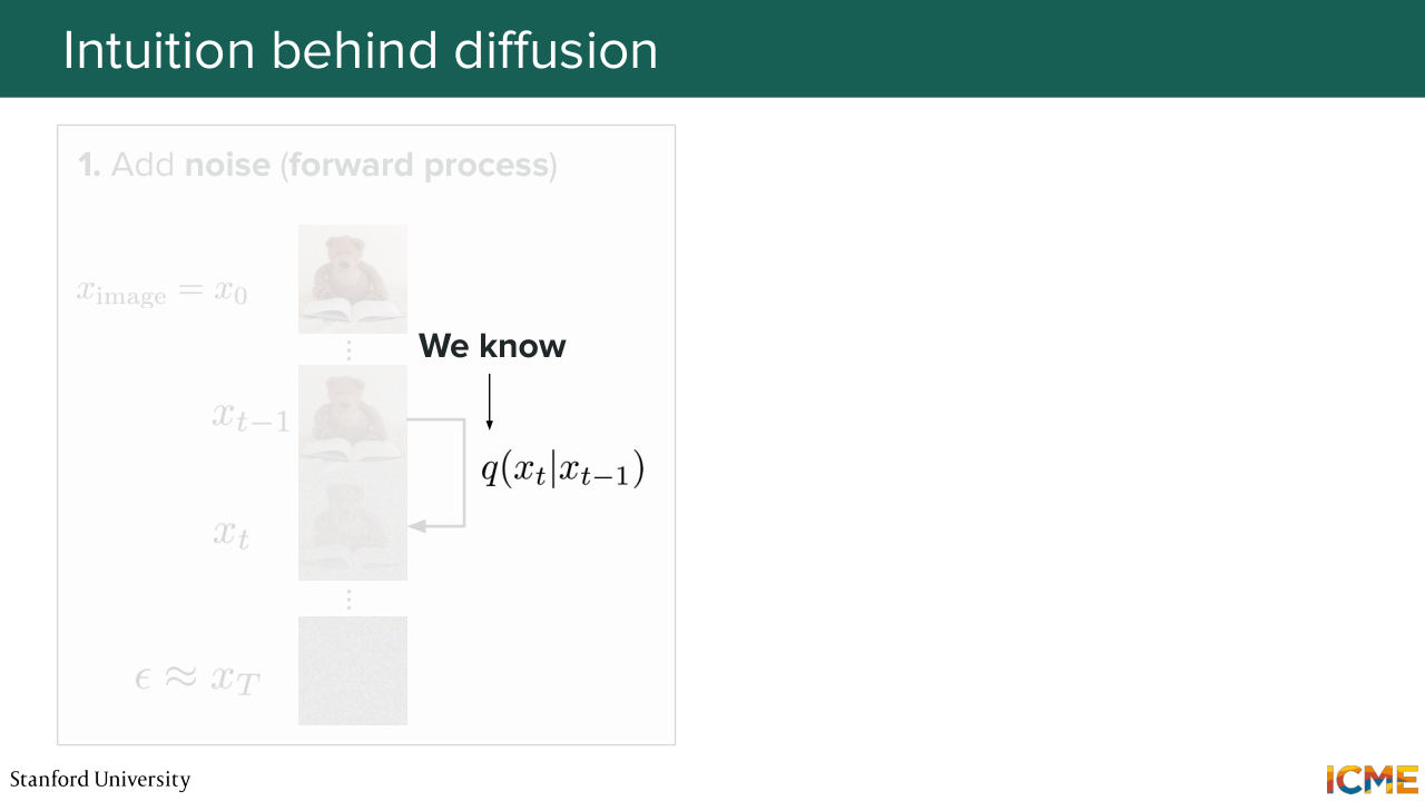
25:22 So here you have some process that you define that goes from some image xt minus 1,
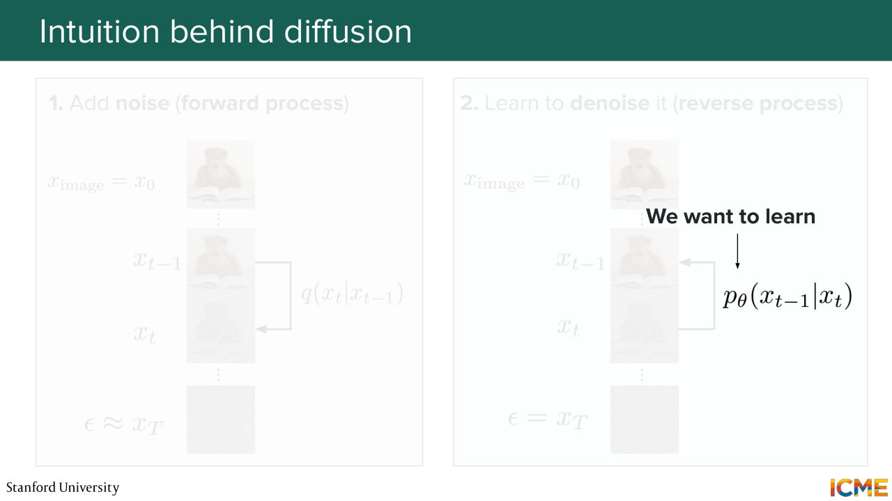
25:33 and then produces an image xt by adding some noise. So again, this is a process that you define. So you know what Q is in the forward process. And what you want to do is to start from that noise distribution that is so easy to sample, and then go through the reverse process
26:01 to actually denoise that sample back to the clean space. And so what you want to learn is a model, that is something we will characterize with the parameters theta-- what you want to learn is how you would go from a noisy image to a less noisy one. So you may wonder, OK, so you're talking about xts,
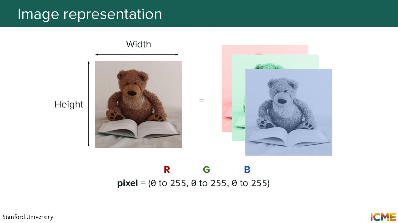
26:40 but we don't what is xt. It's just a noisy image. How do you go about just representing images in the first place? So here we will just see one way of representing images. That is not the way people usually go about it. That's something that we'll go more in depth in lecture 4, but I just want to tell you how you would try to represent images in this framework.
27:09 So as you know, an image is composed of pixels. So you have a height and you have a width. So each pixel is actually composed of three values red, green, and blue, and this allows you to cover a number of colors.
27:33 So based on that, you can represent your image as a function of all the pixels that are composing that image, where each of these pixels contains some value for each of these colors. So you can think of each pixel as having three values, one that represents the amount of red, the other one that represents the amount of green,
27:59 and the other one that represents the amount of blue. So based on that, it is fair to say that you can represent images in a vectorial fashion. So here the dimensionality of the image in this example would be equal to the number of pixels times the number of dimensions you need to represent in a pixel, which is 3. So here you would have n dimensions
28:27 where n is equal to number of pixels times 3. So this would be one way to represent your images. Of course, this is not the most clever way of representing images, and we will see that more in lecture 4. But what I want you to remember is when we talk about images here, when we say x0, xt and so on, what we're talking about is actually vectors.
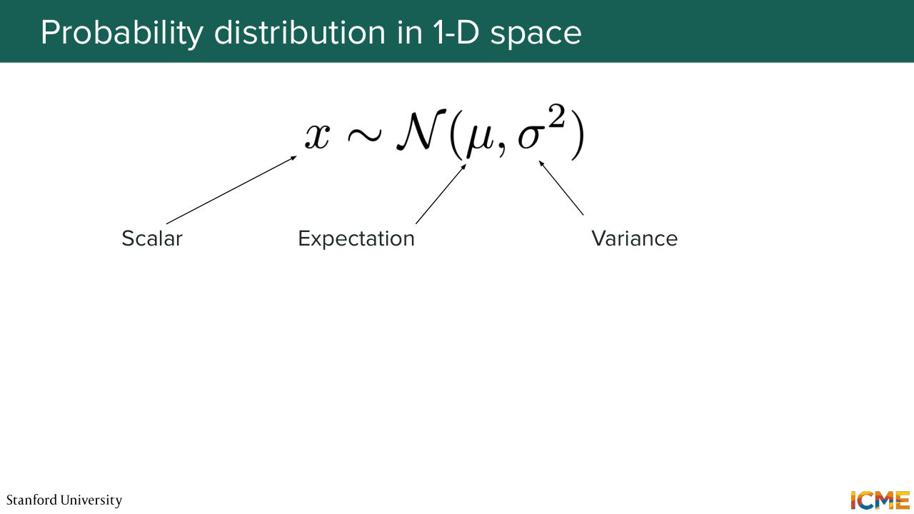
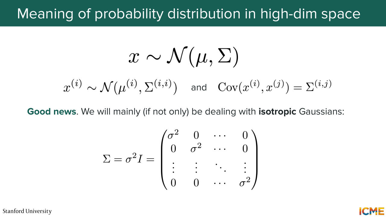
28:55 And these vectors are the ones that are representing these images. Make sense? Cool. So, speaking of vectors. So I told you there is a prerequisite on probability theory, so I'm just going to cover the basics here. So you may know the common distribution, that's called the Gaussian distribution,
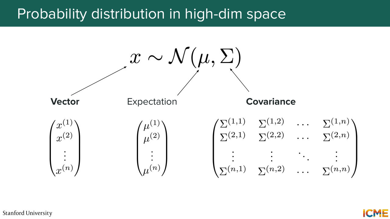
29:19 normal distribution where you have some random variable that is drawn from a distribution of mean mu and then variance sigma squared. Well, you can have the same thing for vectors. So I know all these papers they assume you know that. When you read, it's not super clear, so just want to emphasize. You can also have random variables that are vectors.
29:48 And in this case, you will have a vector that is drawn from a distribution of some mean and the mean is a vector and then some variance, which is actually represented by a covariance matrix. So don't worry if you don't about the covariance matrix, because most of the time we actually simplify the covariance matrix to be a variance times the identity.
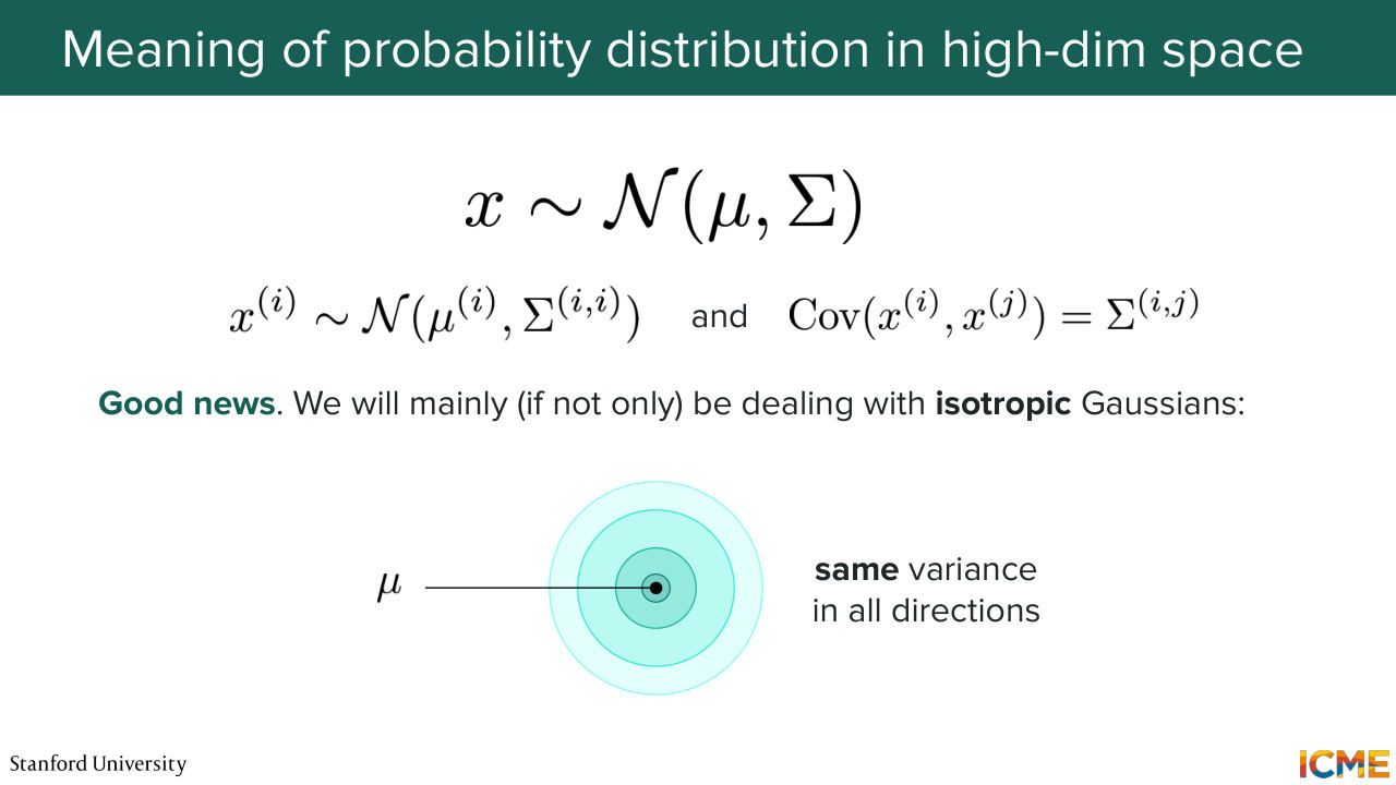
30:21 And we call this formulation actually-- so these are like isotropic Gaussians. Because what that means is that the variation of the data across all directions is the same. So most of the time, to just simplify the math, what we will assume is that the covariance is actually equal to sigma squared i, which is the diagonal matrix which you see here and not the super complicated covariance matrix.
30:53 So by the way, do you remember what covariance is roughly? So maybe I can just recap. So what is covariance? So covariance is a quantity that quantifies how two random variables vary in a linear way. Of course, there is some mathematical expression, but this is like the general intuition.
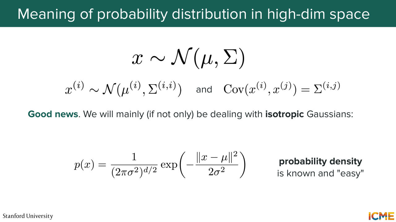
31:18 So speaking of intuition, when we say that a distribution is isotropic, this is what we mean. We mean that the variance is the same across all directions. So you can think of it as some circle where the color represents the density. Yeah. OK, cool. And of course, what's great about Gaussians
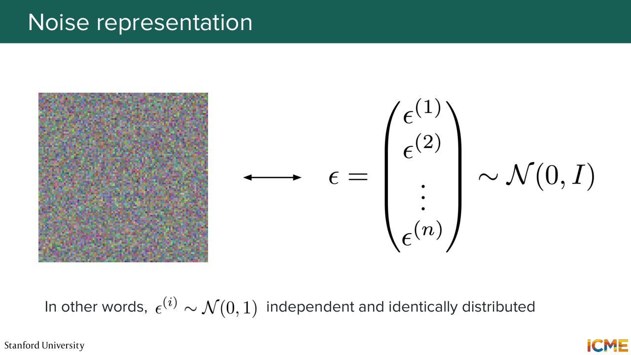
31:49 is you also have an analytical expression that's quite simple about the probability density function. So I'm just putting this here, and it's easy to compute. That's great. So going back to what we call noise. So here we saw that images can be represented by vectors. So when we say we sample from noise, we will say here that we actually
32:19 sample from a standard normal distribution. So we usually note that epsilon. So epsilon will be drawn from a normal distribution of mean 0. So 0 is actually the vector, the 0 vector. And then the covariance will actually be the identity matrix. Yeah.
32:58 It's a great question. It's a great question. So the question is is the representation continuous or discrete? So we talked about pixel values that were discrete 0, 1, 2 until 255. But in practice, these are actually scaled between, let's say minus 1 and 1 or some value that's more of a float. So you can assume that these are actually continuous.
33:23 But you can assume it's actually continuous. Yeah. So there's always some assumption. And so here at least when you say there is no correlation between pixels-- so here we actually mean the noise. So noise we actually just sample at random.
33:51 So yeah, yeah. It's not true for actual images, though. No, it's not true. Yeah, yeah. Great questions. OK, cool. I'm just looking at the time and I know we have a lot of content, so I'll just go a little bit faster. Just want to know if the pace so far is good. Yeah. OK. I don't want to lose you because I think this is the first lecture that is maybe the most difficult
34:18 in terms of math. So it's just kind of sad that this is the first lecture. But yeah, let's continue. So as I mentioned, what we want to do is to take clean images and to corrupt them. So what we do is we take some image that maybe we have noised and we add some noise. And we actually add these quantities
34:44 in a weighted fashion. And these weights are actually defined by us. So if you remember, when we talked about queue, the process that we defined for the forward process, is actually something that we define. So this is how we know it's images. So we take an image. We take some noise from a distribution,
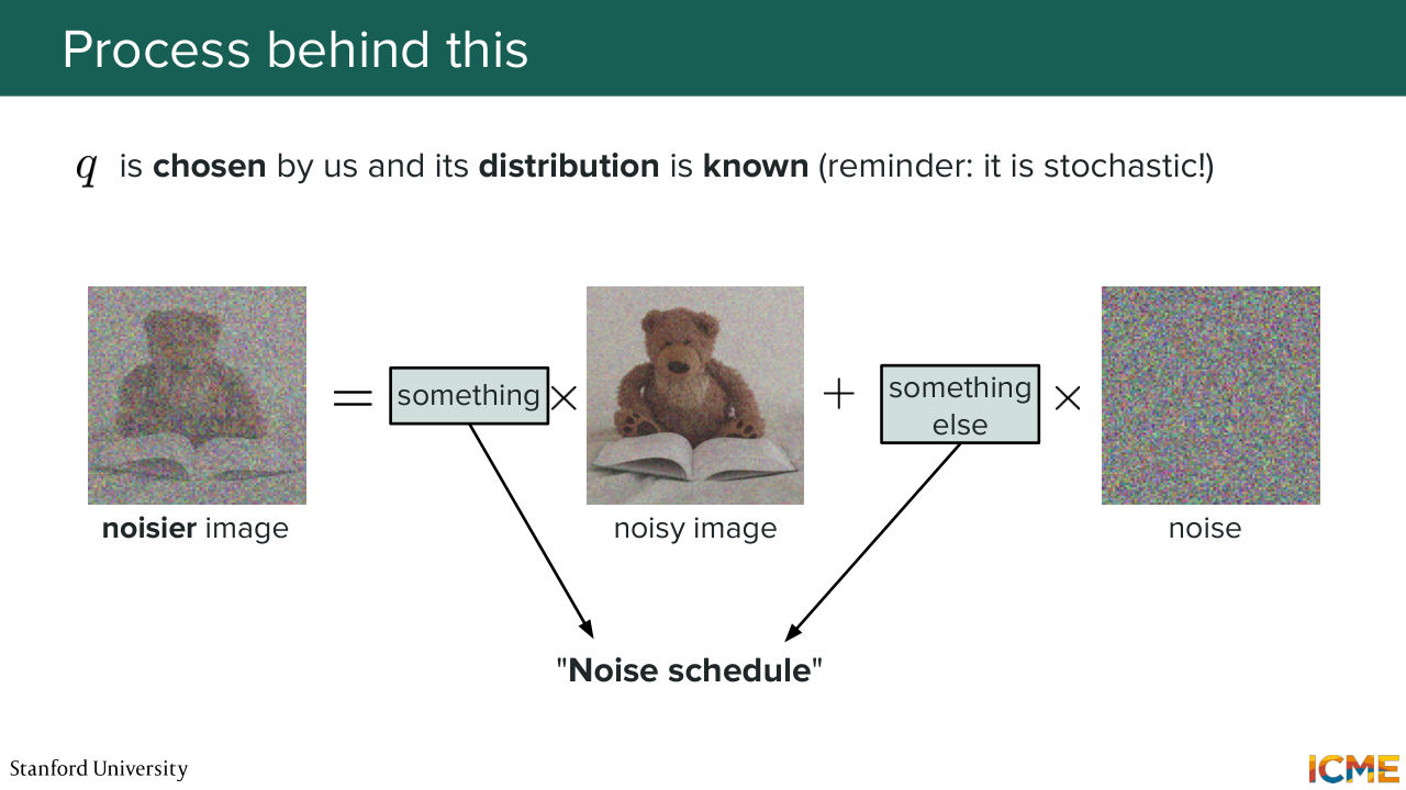
35:12 from the normal distribution and then we do a weighted average with some weights that we will see. And speaking of those, you will hear of a recurring term across all papers, noise schedule. So the noise schedule is actually referring to the coefficients here that you use to multiply these values. So it's a schedule because at some point,
35:39 you may add maybe less noise than some other points. Yeah? OK. Great. So let's go a little bit more into the math. So we start from x0. And then the way we go about adding noise is we have our forward process that we've defined
36:08 q which is actually something we will draw from a normal distribution. So we can express the quantity-- so q of xt, so the noisier image compared to the less noisy image as a normal distribution centered on that less noisy image with some coefficient
36:34 where you add some noise, which is something that is represented by the covariance matrix beta ti. Yeah. So what that means-- I'm just going to rewrite this in a very-- so it's just what that means. So it's xt is equal to 1 minus beta xt minus 1 plus square root of beta and some noise.
37:14 So this seemingly math formula is just nothing else than just you taking your less noisy image, weighting that by some coefficient, and then adding some noise with some coefficient. Now you may wonder why are you using these coefficients? So we will see later in the class why we do that.
37:36 But you can see that the variance of this whole thing is preserved from one step to another. So you will see that this way of noising images is called variance preserving, VP. We'll see that more later on. OK, cool. So speaking of the noise schedule. So these beta t are not typically uniform,
38:06 they're varying. And the way they are defined in the DDPM paper is they're gradually increased. As in you will start from your clean image, and you will just add a little bit of noise, and then maybe a little bit more, and again and again. And then at the end, you will have much bigger noise. And the reason why people do that
38:29 is because when you're close to the clean image, what you care about is to learn those little details, but when you're closer to the noise, what you care more about learning is the general shape of the image. So this noise schedule is actually quite important in our ability to learn and it's just one way of doing things. Yeah.
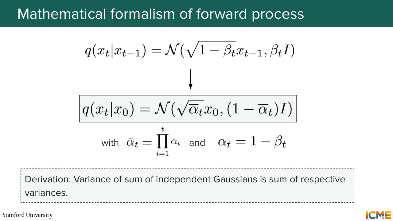
38:57 And as you can tell, it's a between 0 and 1, well, because otherwise you would have a negative value in the square root. Cool. Moving on. So if you define your process like this then it turns out you don't need to noise your images in a sequential way in order to get the number t1. You can actually go directly from your clean image to the step number t.
39:32 Do you see how you would do that? Maybe it's not super obvious, but I told you that Gaussians had very nice properties. So here, epsilon, the noise is drawn from a Gaussian distribution. So if you were to rewrite-- so first of all, I will just define alpha t, which is just equal to 1 minus beta t is just a reparametrization.
40:04 So here it will be 1 minus alpha t. So here what we're saying is xt minus 1 we can also use the same formula, which will be equal to square root of alpha t minus 1 xt minus 2 plus square root of 1 minus alpha t minus 1 and the other Gaussian. So these noise are independent. So if you were to express xt as a function of xt
40:44 minus 2 and the epsilons, what would you do? So here I'm just going to expand xt. So here I'm just in parentheses. So it's equal to alpha t square root of alpha t. So I'm directly going to multiply this quantity by the one that we have here.
41:14 So it's square root of alpha t times square root of alpha t minus 1 xt minus 2 plus square root of alpha t. Square root of 1 minus alpha t minus 1. T minus 1 plus. So by the way, I'm just doing some math. Very basic math. Plus square root of 1 minus alpha t epsilon t.
42:03 So far so good? So here we have our first term. No problem. Then what we have is a weighted sum of random variables drawn from a Gaussian distribution. So I told you that these Gaussian distributions had very nice properties. So it turns out that if you have two random variables that
42:31 are independent and drawn from a Gaussian distribution, so you can really have this as being equal to the standard deviation of this quantity times a random variable that is also drawn from a Gaussian distribution. So how do you add this variance? So you have the variance of everything that is equal to the variance of 1 plus the variance of other.
42:59 So here in terms of how that looks like-- so here, you will have the variance that will be equal to alpha t. So it's basically this squared plus this squared. So it's alpha t1 minus-- 1 minus alpha t minus 1 plus 1 minus alpha t which is equal to-- so this one goes away.
43:27 And then you have 1 minus alpha t, alpha t minus 1. So what does that mean? That means that xt is equal to square roots of alpha t alpha t minus 1. So I'm just like copying what is above. Xt minus 2. Plus the standard deviation of this one,
44:10 which is square root of the variance times a random variable that is drawn from the normal distribution. And this sketch of a proof is just a way for us to prove that you can actually cascade these things up to 0. And therefore you can have an expression of the noisy image at step t as a function
44:49 of the clean image at step 0. And this can be expressed as a function of alpha bar, where alpha bar is equal to the product of the alpha I's. So here alpha t alpha t minus 1 is just the start. But if you continue it's just the product of all the alpha t's. Does that make sense?
45:18 So what I just wrote on the board is just a way for you to be convinced that what I'm saying is making sense. So you can express xt as a function of x0 by just using alpha t bar instead of this beta t. Cool. So yeah. So the derivation you use the fact that the variance of the sum of independent Gaussians is just the sum of the respective variances. And by the way, there's many derivations
45:54 we can do in this class, the problem is we do not have time. So here is the first one, which is why I wrote on the blackboard. But if we do not have time, we will always have a little message at the bottom of the slide that just tells you what the trick is. And you can safely assume that if we don't derive this thing in class,
46:20 it will not be asked during the exams. OK. Cool. Moving on. So now what we have done is just defined our forward process,
Shown briefly — discussed together with the adjacent slides.
Shown briefly — discussed together with the adjacent slides.
Shown briefly — discussed together with the adjacent slides.
Shown briefly — discussed together with the adjacent slides.
Shown briefly — discussed together with the adjacent slides.
Shown briefly — discussed together with the adjacent slides.
Shown briefly — discussed together with the adjacent slides.
Shown briefly — discussed together with the adjacent slides.
46:36 and we just also derived a convenient way to noise our image from step 0 to step T without going
46:45 through all the steps. So what we will do now is to see how we can actually
46:56 go about determining the process that denoisers that forest
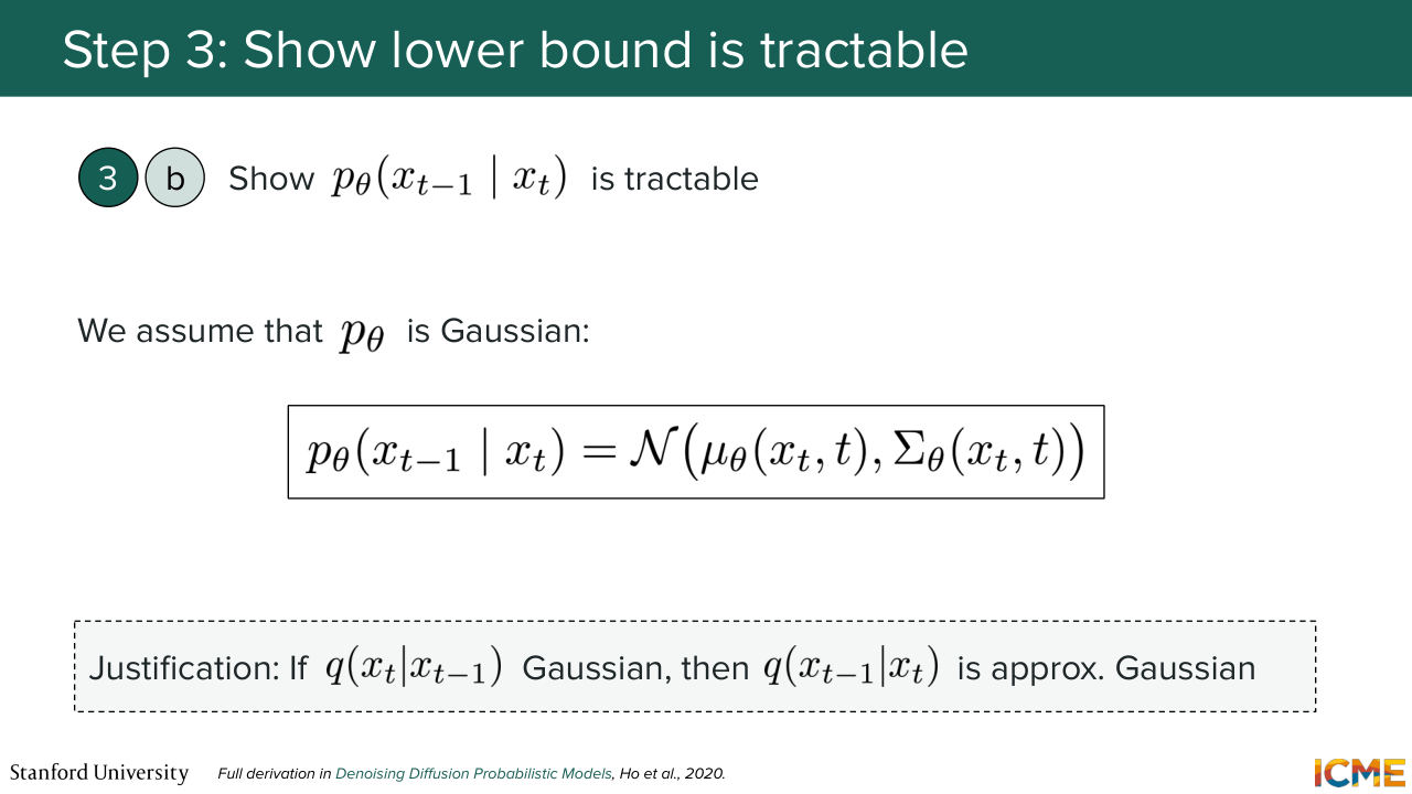
47:01 process. So what we want to is how can we go about seeing what p theta of xt minus 1 given xt is.
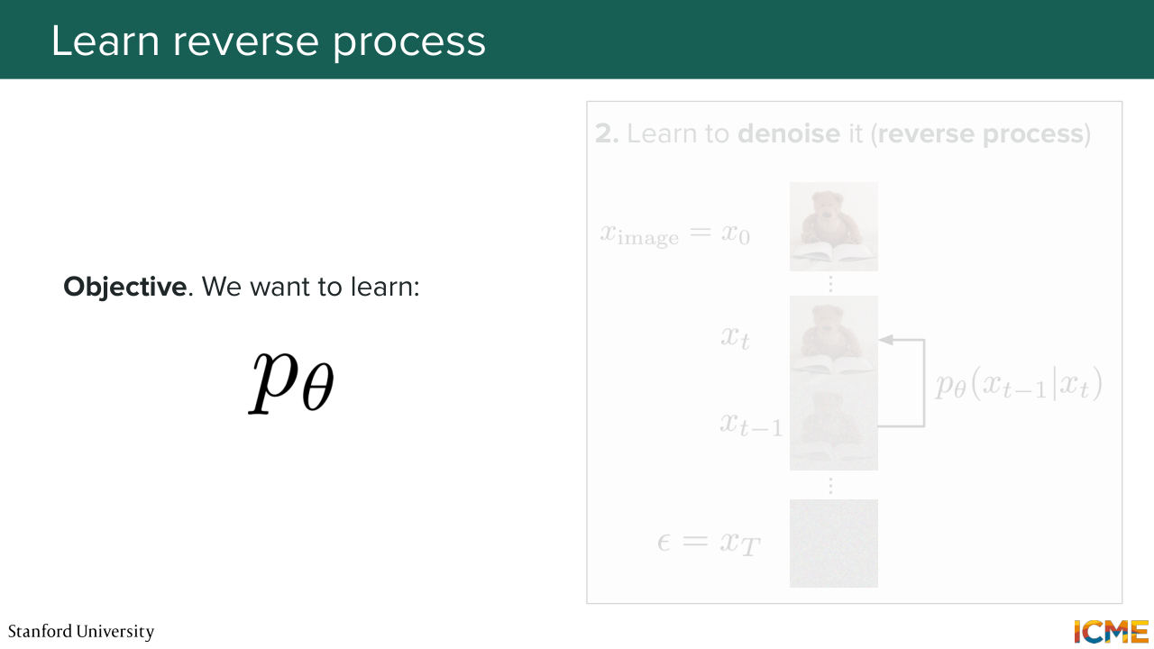
47:15 So as I mentioned, what we want to do is to learn p of theta. So in case you have some experience in ML,
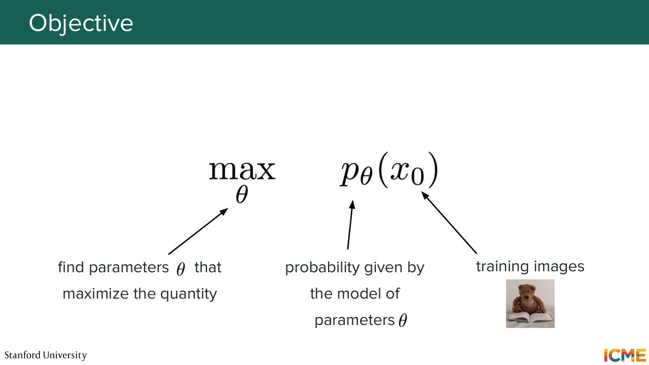
47:26 you will see that a common trick that people do is given some training data what they want to do is to maximize the probability of your model seeing the training data maximized. They want to maximize such a probability with respect to theta. So they want to find the parameters theta that maximize the probability of your model of seeing your training
47:58 data. So in this case training data is just our training images. So it's clean images. And then our model here is something that has p theta in it. So it's the probability of an image happening that we will see how we can condition. And what we want to do is to find the parameters theta that do that.
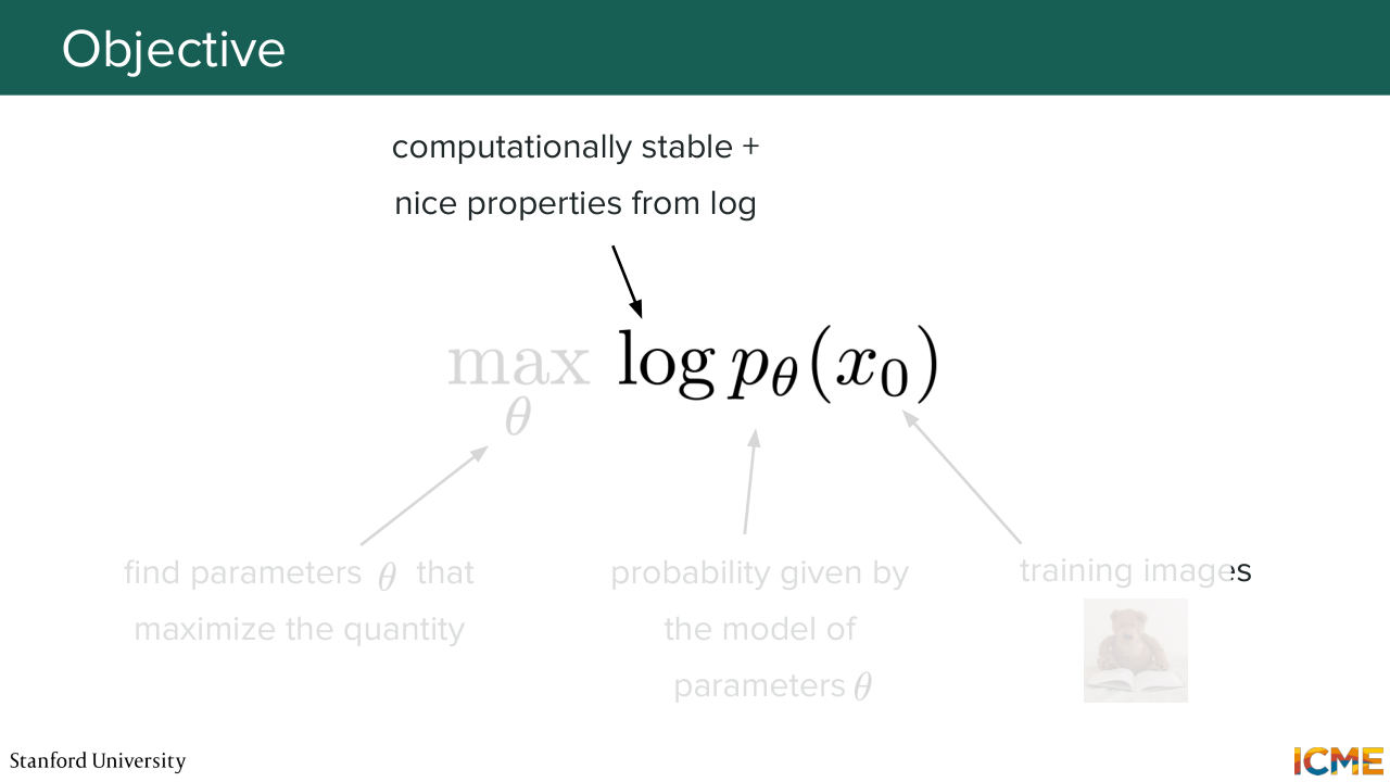
48:25 So you will see that whenever you talk about probabilities, you will always or most of the time talk about log probabilities. One because the logarithm function has pretty nice properties. And then the second reason is that it's just computationally more stable, because probabilities are between 0 and 1.
48:50 So if you have very, very small values of p, then it can be a little bit unstable.
48:56 So before we determine that, I just wanted to go through some refresher of a concept
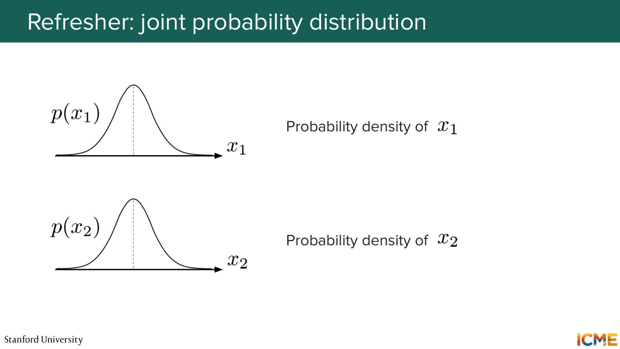
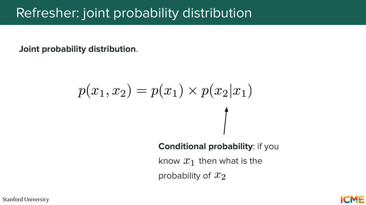
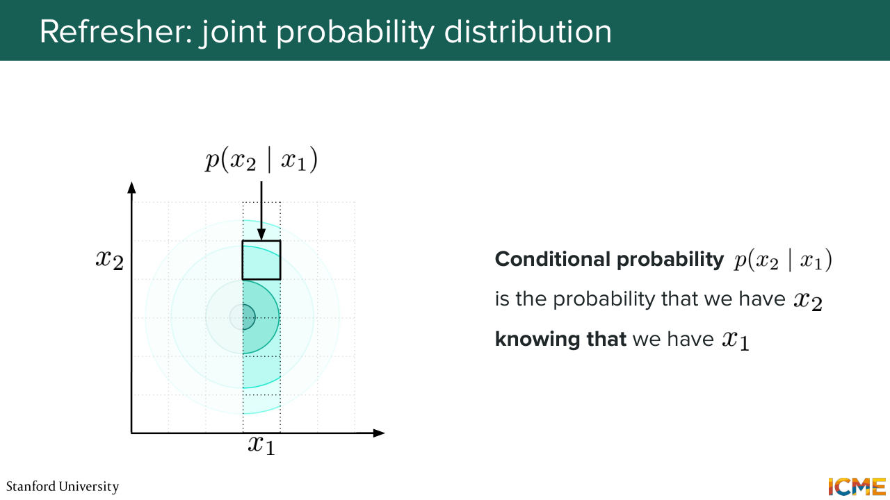
49:06 in probabilities that is the joint probability distribution. So here if you suppose that you have two random variables that are drawn from two distributions, let's say it's x1 and x2, the random variables, then you can compute the joint probability distribution,
49:33 by taking the probability density of x1, and multiplying that by the conditional probability of x2 given x1. So this is just by definition, it's the probability chain of rule. And in practice, when you have a joint probability distribution, one way you can represent that is through a heat map. So here you have, let's say, your two axes.
50:08 One is representing the one along x1 and the other one along x2. And then here the color that you see here is the density value of this joint probability distribution. So this is for instance 1 square.
Shown briefly — discussed together with the adjacent slides.
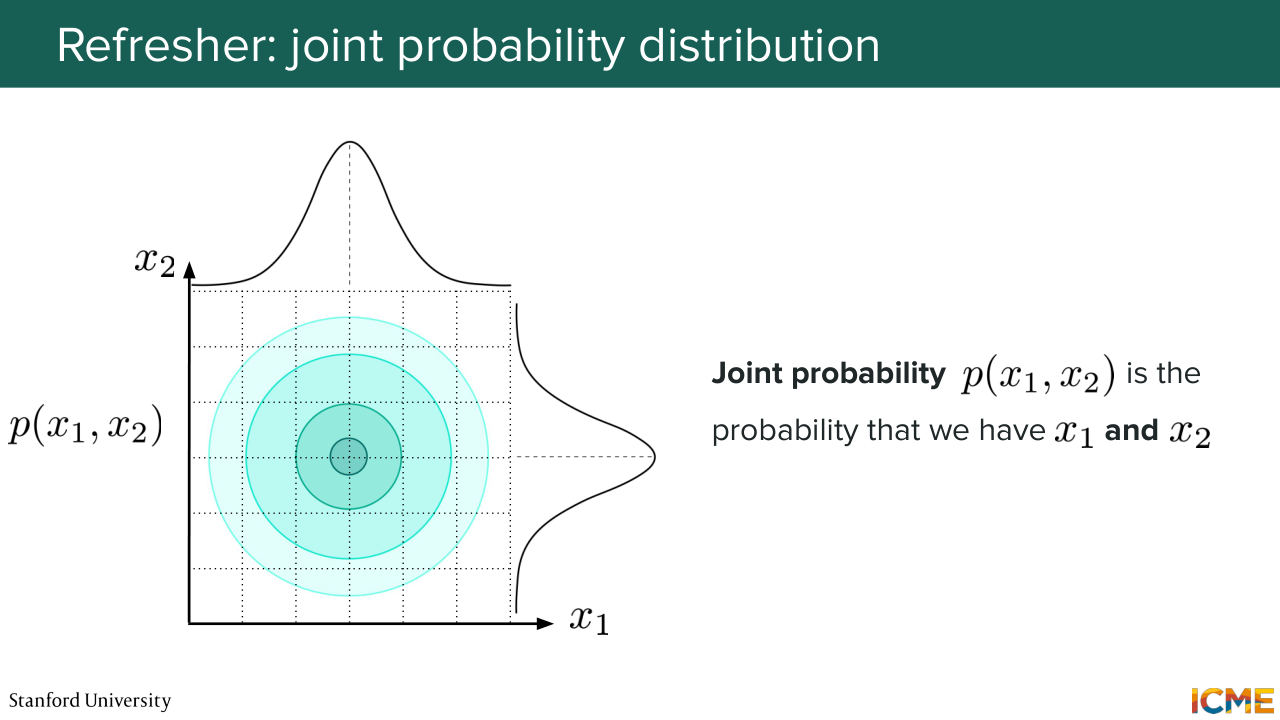
50:33 And the way you would go about doing this for the conditional probabilities you would actually just look at one column. And here the probability of x2 given x1 would be the proportion of the value of the joint probability distribution in that square over the sum of all the squares for that given value x1. So far I'm just recapping what we
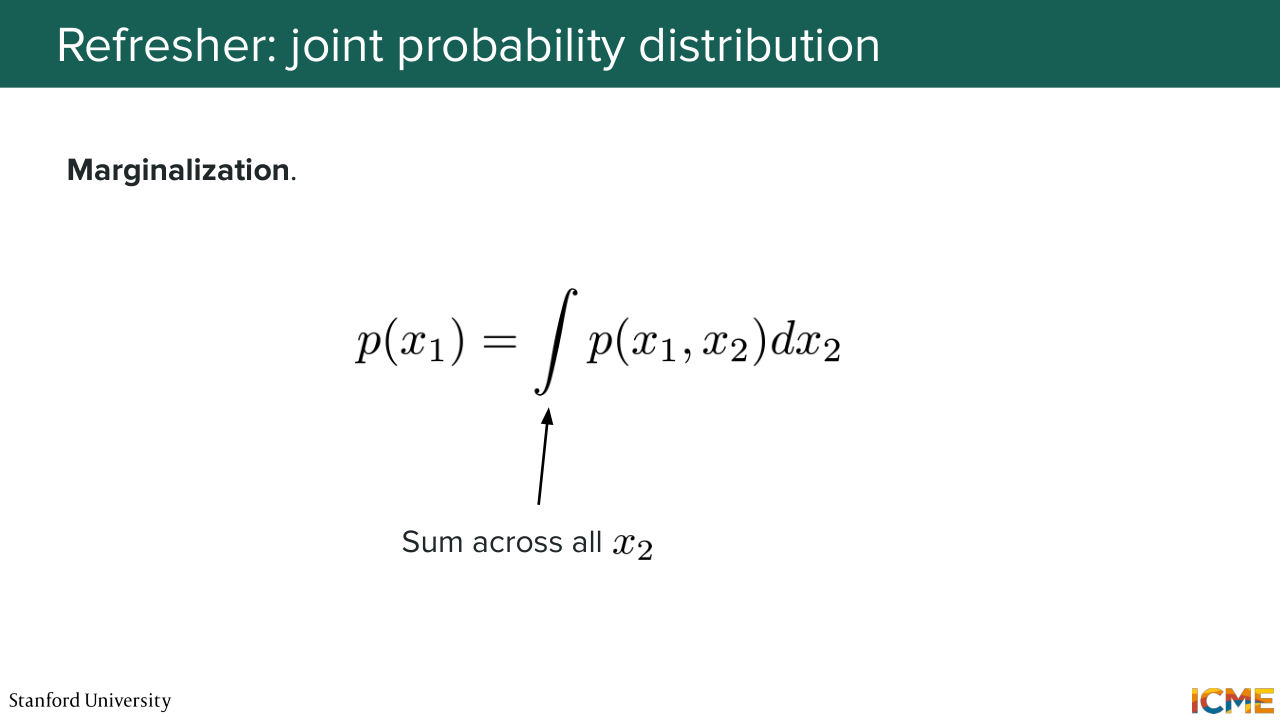
51:05 know about joint probability distributions and conditional probabilities. So what I want to tell you is a notion of what we call marginalization, which is if you want to obtain
Shown briefly — discussed together with the adjacent slides.
Shown briefly — discussed together with the adjacent slides.
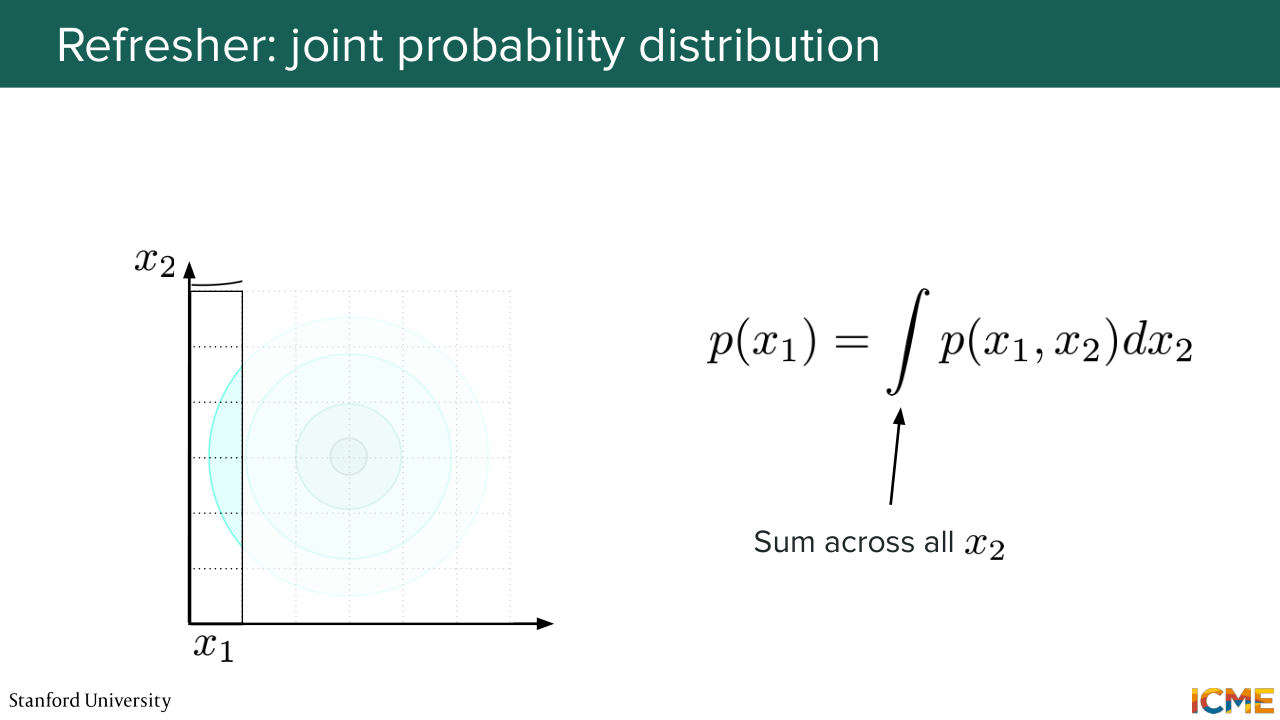
51:24 the probability of just one random variable, then what you can do is to sum the joint probability of that random variable and a second random variable, and you can sum it along that second variable. And this is called marginalization. Do you all know-- have you all heard what marginalization is? Yeah? OK, cool. So what I'm saying is a little bit obvious then.
51:57 So in this figure so the way you would obtain p of x1 is you sum all the squares relative to x1 again and again and again and you can reconstitute your probability distribution. So that's the way you would see this from a graphical perspective.
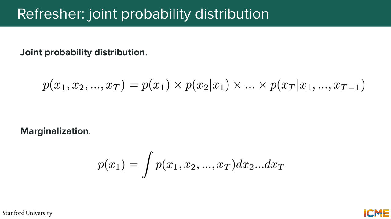
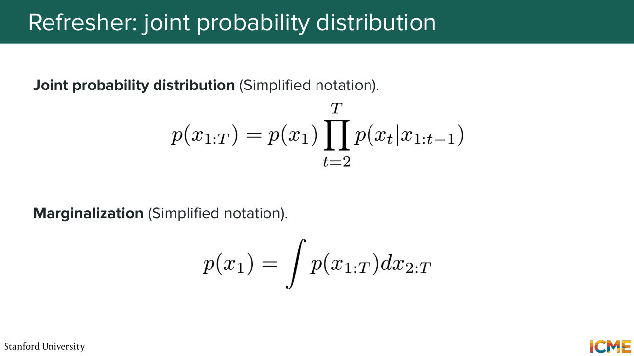
52:24 And so we saw that when we only have two random variables, but you can very well do that when we have T random variables. And so here we have the probability chain rule like at the top of the slide. So you have p of x1 times p of x2, given x1 et cetera times p of xt given x1 up to xt minus 1. So this is just extending that to a dimension of t.
52:58 And one notation that you will see very often in papers is this one. So the joint probability distribution of T variables is usually denoted p of x1t. So just to save space. And the reason why I'm presenting these slides
53:23 is just to tell you that this is the main notation that people use and this is what it means. Cool. And with that simplified notation, you can just rewrite the formulas from before as follows. So now if we were to come back to the problem that we had around finding parameters theta that maximize the probability of our models seeing the training data.
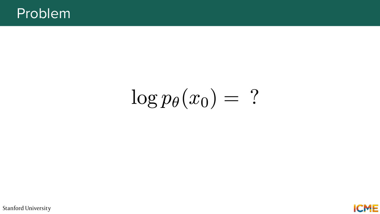
53:58 Here, what we want to do is to express p theta of x0 or log of p theta of x0. So we've seen a few slides ago that the way we obtain x0 is sampling from a noise distribution at time t. And then going step by step from big t to big t minus 1,
54:26 et cetera, up until 0. So in order to compute this quantity, one idea for you could be to take the joint probability distribution over all the time steps and then sum across all these different quantities except x0. A.K.A. you can just marginalize, right? So one idea is to say that the logarithm of p theta of x0
55:05 is the logarithm of the integral of p theta of x0 and then x1 up to t. D of x1 to t. So this is just the definition of marginalizing. So the problem with this formulation is that it's actually something we cannot compute because here
55:34 we're saying let's marginalize-- let's sum across all possible trajectories from noise to clean image. So the problem is there are many of them. And these x's we saw that these are vectors,
55:54 and they can be pretty big. So long story short, is this is in practice something that we
56:01 cannot compute. Which is the reason why we have a recipe that we will go through
56:10 in the next 33 minutes as to how we can compute that using the forward process
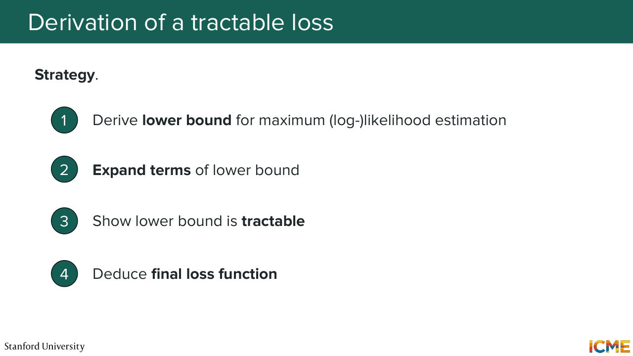
56:18 that we have defined. So in the interest of time, I'm going to skip some blackboard derivation, which is fine. I'm just going to give you the trick. If time permits we can do a few ones. But the important thing for you is to just understand the high-level strategy around obtaining the loss that will be used to train our model.
56:45 Sounds good? Cool. So let's start with the first step.
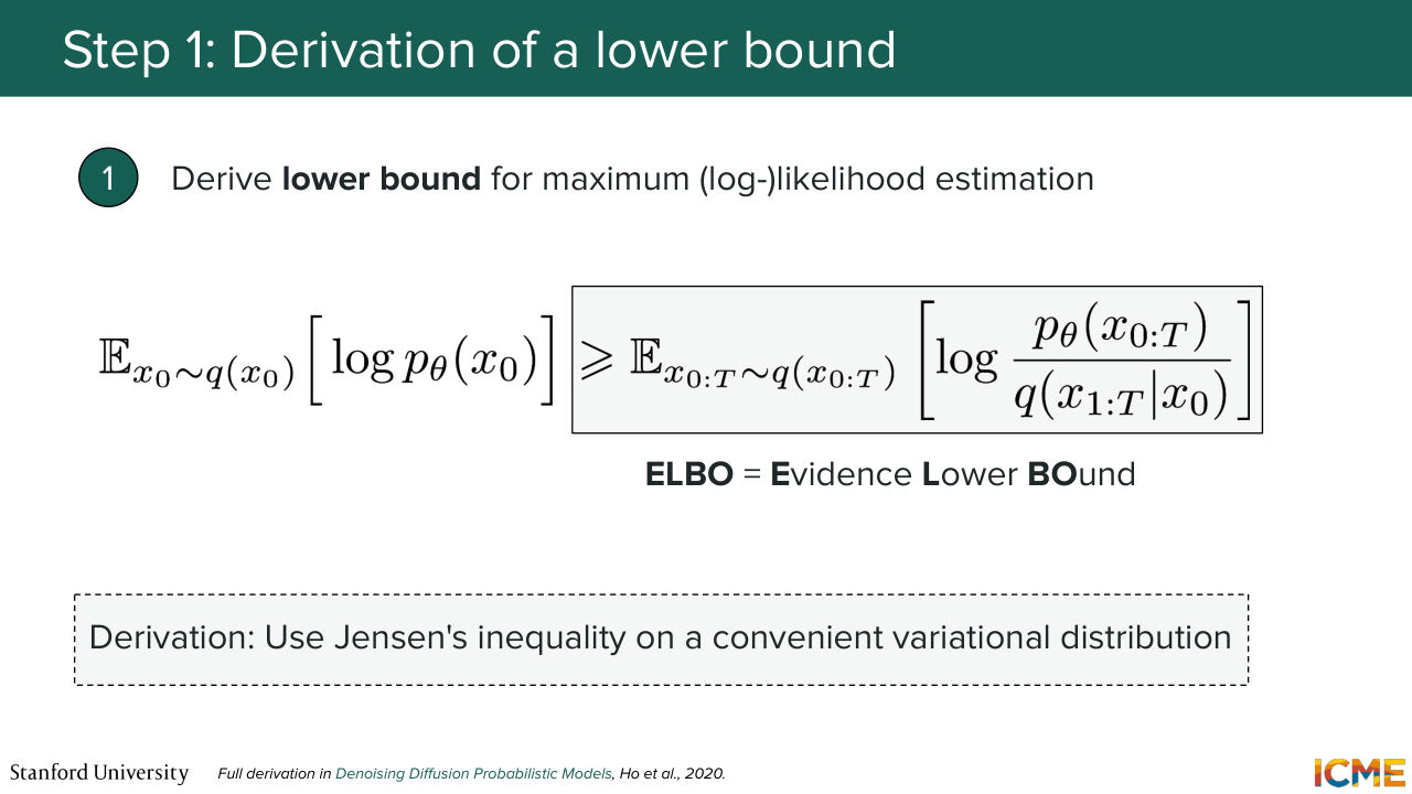
56:52 So I told you that this expression is something that is actually not something we can compute because it's just intractable. So a common trick that people use is to find something that is easy to compute that is not necessarily the quantity of interest, but maybe a bound that is close to what you want.
57:23 So here what you want is to maximize that expression. So if you were to maximize something that you know is lower than that, so a lower bound, then it would also allow you to gain some confidence that you're maximizing the right thing. So there is a very scary formula on the slides
57:44 which we'll go through right now, which is the elbo. Have you heard of the ELBO before this class? Yeah. ELBO stands for evidence lower bound. And what that means is it's an expression of a quantity that is a lower bound of the quantity that we care about. And actually, this is quite important, so I think I will derive it.
58:14 So while I'm cleaning the blackboards, I just want to tell you about what the trick is. The trick is that we have our forward process that we have defined, so q. And what we want to do is to have q be in some way something that we appear. Like in our equation, we want to involve q in some way
58:46 because what Q is. Q is this forward process that we have defined when we do the noise schedule this beta t alpha t, we know that. So what we want to do is to express that as a function of q. So we go back with the log of p theta of x0, which we said we tried to marginalize across x1 to xt.
59:17 So I'm just going to rewrite what we had above. And then what I'm going to do, as I mentioned, is have q appear. So very common trick. What I'm going to do is to multiply the numerator and the denominator by that quantity. So I'm going to do this one times q of--
59:55 So given a clean image, what is the trajectory that is given by q? So it's q of x1 to xt given your clean image. OK. Everyone is following me so far? Just a very regular trick. So OK. So where do we go from there? So I'm just going to remove the log for now.
1:00:34 So this is true. So this expression is actually nothing else than the expectation of this quantity because this is as if you were sampling x1 through T from this distribution. So it's as if you were writing this.
1:01:15 So it's as if you were saying it's the expectation of this ratio, which is p theta of x0 to t over q of x1 to t, given x0, where x1 through t is something that you draw from q of x1 through t given x0. OK I hope-- so don't worry by the way. It's all going to be in the recording. It's going to be much clearer in case you cannot see very clear
1:01:53 what I'm writing, but what I'm writing is the expectation. This quantity is the expectation of the ratio between p theta of x0 to t over q of x1 through T, given x0 by sampling x1 through t-- so the trajectory through t via the forward process that we know, which is given by x1 through t given x0.
1:02:23 So where do we go from here? So it turns out that there is a very common trick-- very common trick out there that's called the Jensen inequality where if you have a convex or concave function, you have some very nice property about something we're going to see. And in particular, in this case, log is a concave function.
1:02:57 So if you have the log of some expectation, it's actually something that is greater or equal than the expectation of the log. I'm not going to write this whole thing, but you know what I mean. So this is Jensen's inequality. Jensen.
1:03:33 And this is exactly what we get here. So one way we progressed is instead of summing through all possible trajectories, now what we're doing is we're actually sampling from trajectories that were drawing from the forward process, which we know.
1:04:00 And now you're wondering why in the slide are we sampling x0 through T. But here I said x1 through t sample from q of x1 through t given x0 is because if you take the expectation of this whole thing, then you take the expectation over x0 of expectation of x1 through t times that. So you use the chain rule of probability
1:04:33 that we saw right before. And it's exactly the same. Just one expectation of sampling the whole joint probability distribution through this q x0 through t.
1:04:48 Does this make sense? So you may see this formula and wonder, OK, it's still super complicated, how can I compute that. Well, right now, you do not know that it is tractable. I'm just telling you. But the intuition here is we're actually not summing through all possible trajectories. We're actually summing through trajectories that we're sampling from the forward process.
1:05:21 Yeah? So now it's step number one. Step number 2 is proving or showing
1:05:30 that this is something that you can compute. But before that, I'm going to, again,
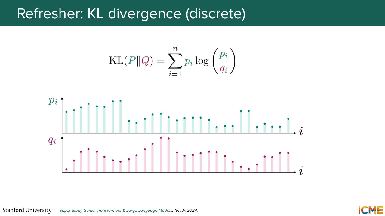
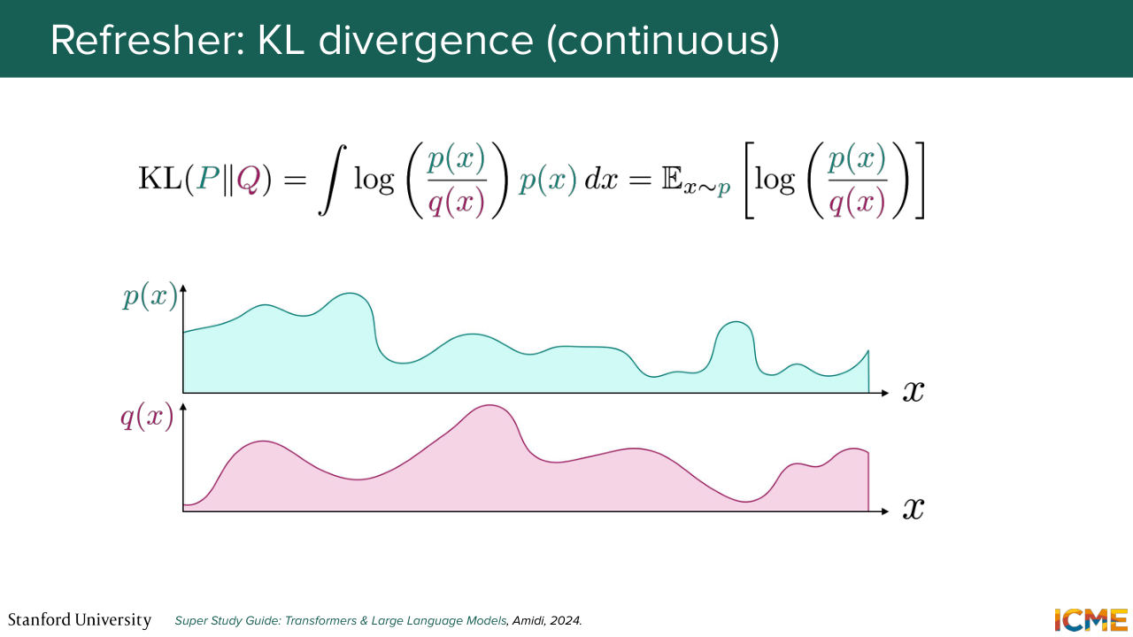
1:05:36 give you some refresher of a very important concept that is the KL divergence. Who has heard of KL divergence? Yeah, everyone? I'm just going to remind you what KL divergence is. So if you take two probability distributions-- so let's say p and q-- and you want to measure how far apart they are, then
1:06:03 there is some operator that is here, the KL divergence, which quantifies how far apart they are. And the way they do that is by taking-- maybe it's something I treat on the slide. So I'm just going to continue their. So by taking the sum of the log of the ratio between these two probabilities weighted by the probability distribution p.
1:06:42 So in the discrete world, it's going to be like this. But we're going to be mostly in the continuous world. And in the continuous world, the KL divergence is this, but in integral form. And it's the same as saying you take the expectation of the logarithm of the ratio if you were to assume that x is sampled through p.
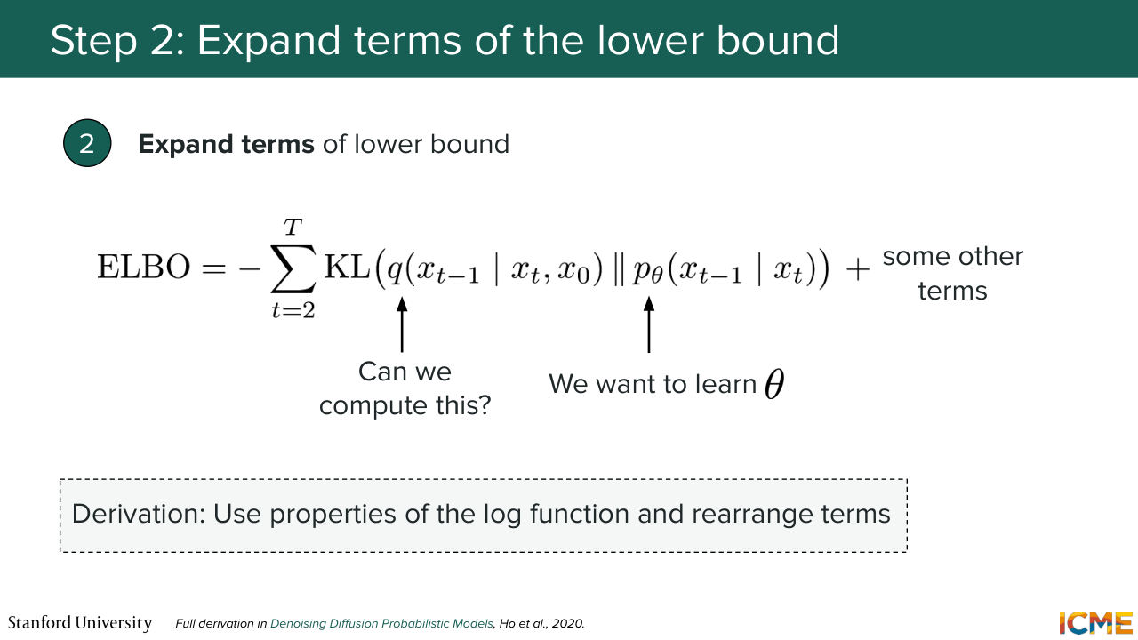
1:07:11 Yeah? OK. So given that, we can prove that the ELBO term that we saw-- so you know this lower bounds here, it can actually be expressed with terms-- so some terms that we actually don't really care and we're just going to ignore-- plus a term here, which is the KL divergence of q of xt minus 1 given xt and x0.
1:07:47 So it's the first distribution. And the second distribution is actually the probability of having the less noisy image xt minus 1 given xt, which is the thing that we want to learn. So we don't have time to derive this, but it's actually not that complicated of a derivation.
1:08:15 You would just take this expectation of log, and then you would do some manipulation here and there, and you can basically pop up the KL divergence operator through that. So I think this one, I will need you to trust me that this is equal to this. So why are we happy? The reason why we're happy is because we
1:08:43 have a clear comparison between two probability distributions,
Shown briefly — discussed together with the adjacent slides.
1:08:48 one that we care about, and another one that is potentially something that is tractable.
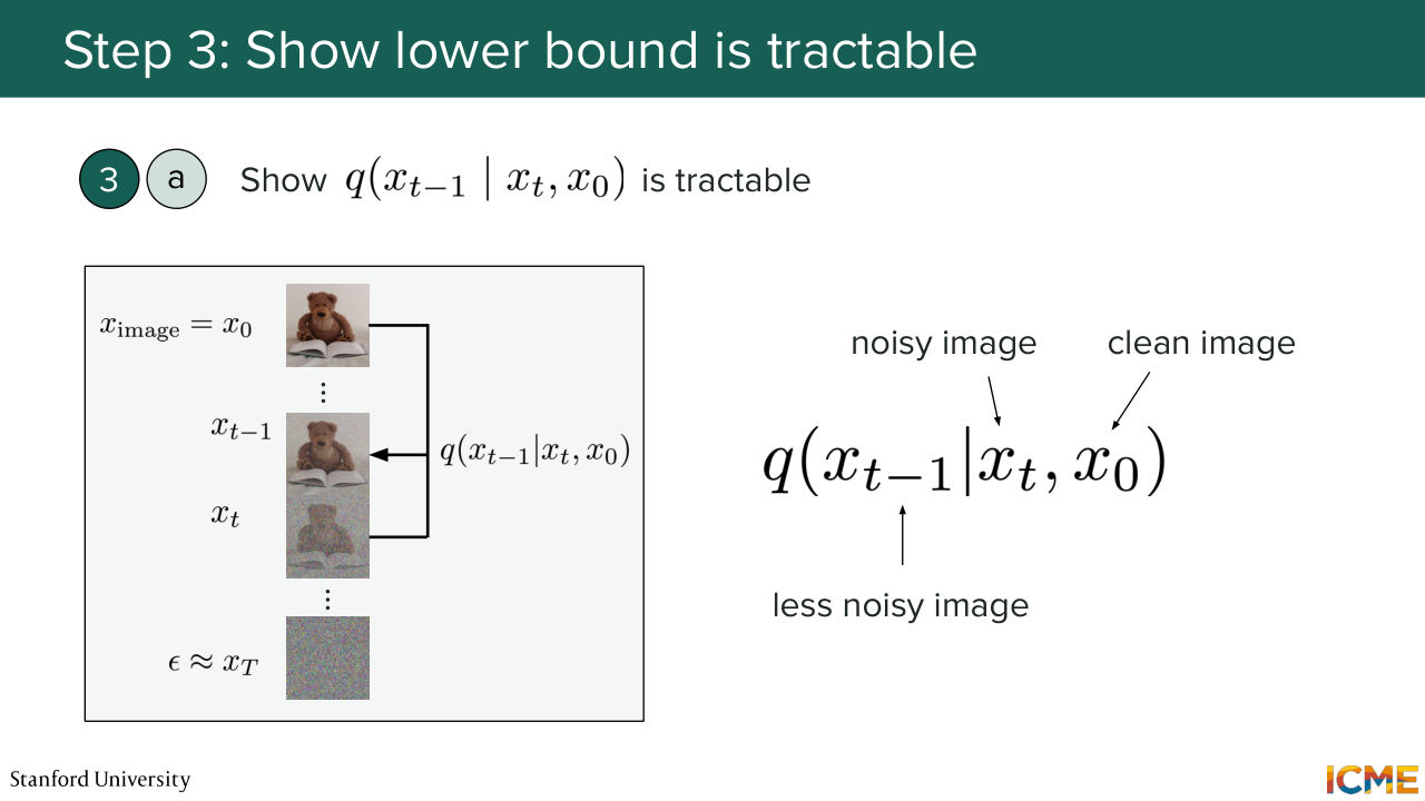
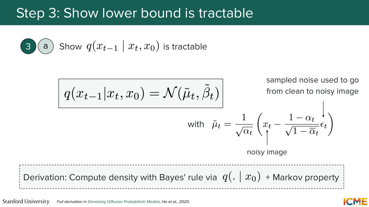
1:08:56 And so just to tell you what q of xt minus 1 given xt and x0 means, so it means that if I were to give you a noisy image and a clean image, my question for you would be, what would be the less noisy image if I were to give you this tool. So the good thing is that at training time, you know x0. So you can compute this quantity.
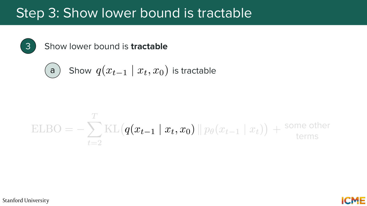
1:09:30 So a natural step for us is now to show that this quantity that I mentioned is indeed tractable. So we're going to see what q of xt minus 1 given xt and x0 is. So again, it is the fact of wondering
1:09:55 what is the distribution of the less noisy image if I were to not only give you the more noisy image, but also the clean image, which is actually a lot of information.
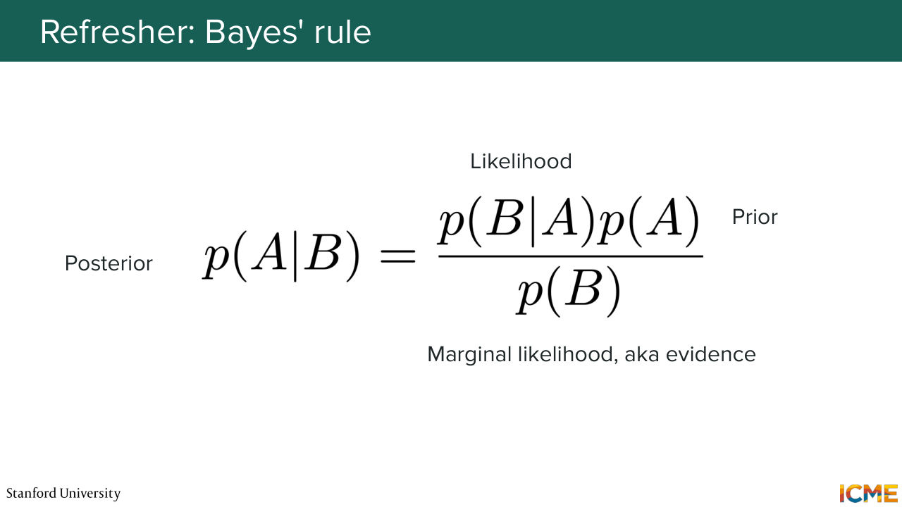
1:10:09 So you may remember, or you may have heard of Bayes' rule.
1:10:15 And it is something that we will use, a trick we will use here. So using the notations that you would commonly see and read and hear out there, it's the fact of saying that the posterior is equal to the likelihood times the prior over the marginal likelihood. So in this case, it's P of A given B equal to P of B given A times P of A over P of B.
1:10:49 And so knowing that, it's actually quite easy to show that this thing is tractable. So this is probably something we will derive. So here, so what we want is q of xt minus 1 given xt and x0. So if we were to use Bayes' rule with q
1:11:30 of the conditional probability based on x0 if you have this formula-- so if we were to write this by considering p equal to q conditional on x0, what we would do is-- so what I'm doing is just applying Bayes' rule. So it's equal to q of xt given xt
1:12:01 minus 1 x0 times q of xt minus 1 x0 over q of xt given x0. You all agree? I'm just doing Bayes' rule. So it's something that I have not told you so far. But q has a very special property. Q is Markovian. So what does that mean? It means that q of xt, given everything before--
1:12:52 let's say before-- is actually equal to q of xt given xt minus 1. In other words, you only need to know about the previous step to know the current step. So it's called a Markov process. So this simplifies to q of xt given xt minus 1.
1:13:18 And then we saw before that q of xt minus 1 given x0 and q of xt given x0 are quantities that are tractable. They are this normal distribution. Do you remember this derivation I made with, OK, let's replace xt minus 1 as a function of xt minus 2 until getting x0? Do you remember? So these two quantities, they are tractable. This is tractable, this is tractable. Actually, this one, we don't really care because we want to compute q of xt minus 1 given xt and x0.
1:13:58 So here, we're only varying xt minus 1, but q of xt given x0 everything is fixed. So you can interpret that as a constant. And so what we end up with-- I cannot do that. Yeah.
1:14:27 Are you referring to this one? The left hand side. So here's the thing-- in this derivation, the quantity that we actually care about is q of xt minus 1 just given xt and x0.
1:14:52 So this is just because of the derivation of the elbow, the fact that we end up here. And that's just the fact that we just are interested in what is the distribution of the less noisy data if we what the noisier one is and the clean image is. That's the thing that we care about. And so here, what I want to say is that this is something--
1:15:25 so x of t minus 1, knowing xt and x0, is proportional of q of xt, given xt minus 1, times q of xt minus 1 given x0. This is Gaussian. This is Gaussian.
1:15:58 The product of probabilities of Gaussian is a Gaussian. I'm not going to derive everything, but please trust me that the form of q of xt minus 1 given xt and x0 is a normal distribution in particular with the mean of this formula. I'm not going to read it, but it's a function of the noisy image and then the sampled noise
1:16:27 that allows you to go from x0 to xt. So this distribution is exact, meaning we have not approximated anything. And this is something that we know because we have defined our forward process. And here, we're cheating a little bit because we're saying, what is the less noisy distribution if I
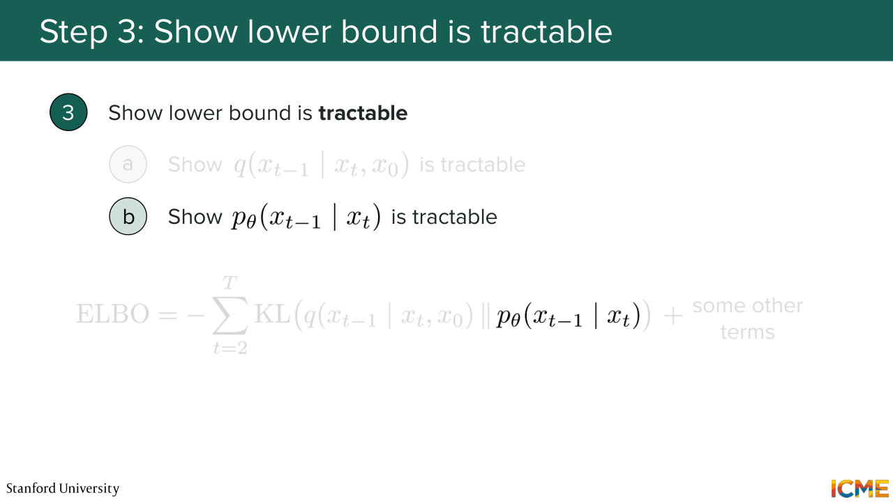
1:16:53 give you the more noisy one, but also the clean image. So it's a little bit of cheating because at training time, we know what x0 is. Of course, at inference time, we do not. So know one term. The second term is this p theta of xt minus 1 given xt. Now let's show that it is tractable. Well, that one is going to be easy because we
1:17:21 can choose what p theta is. And turns out that it's very fair for us to assume that it is also a Gaussian just because the forward process of xt minus 1 given xt is also approximately a Gaussian. So justification for that is a little bit more into the weeds. So I'm not going to go into that. But all of that to say that in this part,
1:17:52 we're just making the assumption that what we want to learn is a Gaussian. So what we end up with is a KL divergence of a Gaussian with a Gaussian. And I'm not sure if you remember,
1:18:16 but early in the lecture, I told you that we know the probability density function of a Gaussian. We have the explicit formula. We do know. So if you replace these into the KL divergence formula, which is this integral of log of p over q and then p,
1:18:42 then it turns out you have a lot of things that simplify. And at the end of the day, what you end up with is just the distance between the noise that you want to predict and the noise that you sample to go from the clean image to the noise image. Take the L2 distance of that.
1:19:13 Is everyone clear with that transition? So what we did was we had that elbo elbow, which was equal to this KL divergence term. And what we said was, OK, looks good because p theta is what we want to compute. And then this q thing is something we have defined. So let's try to see if it's tractable. And what we said was, OK, let's see
1:19:41 if q is tractable, q of xt minus 1 given xt and x0. So we went into the math. We did the Bayes' rule. And then there is this latter derivation around actually determining the mean and the variance of that normal distribution that I've not covered just because it's just too much. And it's OK to just assume that if you do this at home,
1:20:03 you end up with a normal distribution of this mean. And then we also showed that p theta is something that is tractable. And the way we have shown that is just by assuming that it is a Gaussian. So Gaussian of some mean and then some variance.
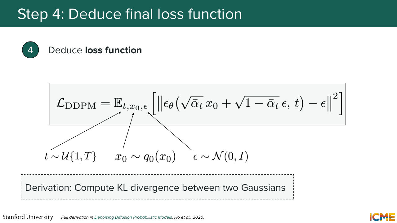
1:20:27 And at the end of the day, we end up with a loss that is nothing else than an L2 regression on the noise that we have added to our clean image to obtain the noisy image. Do you agree that that loss is looking pretty good? It's very tractable. You just have to regress your noise on the noise from the clean image
1:21:00 to the noisy image as a training loss. It's great. Oh, yeah. Thank you. So the question is, what is epsilon theta. So I'm going to go through each term. So here, what is shown on the slide is loss of DDMP. So DDPM is this whole framework of defining a forward process in order to determine how you want
1:21:32 to reverse the process, which is why it's called LDPM. And what is on the right hand side of the equal sign is an expectation over t that you sample, which is the noise level if you want, x0, which is clean images in your training set, and then epsilon is random noise that you sample
1:22:02 from a normal distribution. Sorry, standard normal distribution, which is basically a Gaussian of mean 0 and variance the identity matrix. So what is in the expectation is on the one side, Epsilon theta, which is your model predicting what noise was added, and then on the right side is epsilon, which is the actual noise
1:22:32 that you added from the clean image directly to the noisy image. And what is in the parentheses? So square root of alpha t bar x0 plus square root of 1 minus alpha t bar epsilon-- this is equal to xt. So it's the noisy image because you can go from the clean image
1:22:58 and epsilon directly to the noisy image with using the identity that we have seen. So in other words, it is saying, if I give you the noisy image, please compute the noise that was added and compare that to the actual noise that was added. So one thing that I will call out is there are actually two arguments. You not only give the model the noisy image,
1:23:30 but you're also giving it the information of how noisy it is. T. So here, t is between 0 and big t. So if T is more towards 0, it means you didn't add a lot of noise. And if t is more towards big T, it means you've added much more noise. So it just allows the model to know, given this noisy image, how noisy it is. So it can calibrate how much noise to predict to remove.
1:24:04 Does that make a bit more sense? Perfect. So yeah, but great question. And we're actually going to go through exactly what that means in practice if we want to train the model. But before we do that, any other questions on the loss? Yeah. So the question is this loss represents the elbow. So we are actually going to see exactly how we went from the first step to this step in the next slide.
1:24:38 So I'm going to answer a question right now. So apart from this any other questions on this? We're good? So I'm going to answer your question now. So do you remember the strategy plan we had with these four steps. So we went from this maximum likelihood estimation problem that we wanted to perform. And we said we have a lower bound.
1:25:10 So that's where the elbow comes then from the elbow, which is a lower bound of what we care about, what we said was actually expand the terms. And we were like, oh wow, we actually have a KL divergence between two things that seem tractable. And then what we said was, OK, so let's look at that KL divergence term. There are two parts to it.
1:25:36 One is q of xt minus 1 given xt and x0. The other one is p theta of xt minus 1 given xt. We saw that these two terms were tractable. They were Gaussians. And we knew what the mean of these two Gaussians were. And then what we said was we have two Gaussians. We know their probability density functions. We have a KL divergence of that. Then we can actually compute this whole thing analytically
1:26:10 and, as a result of that, end up with a loss that's very simple. Now there is something that I simplified that I've not told you yet, but I'm going to tell you now. When you simplify this scale divergence, what you actually get is the expectation of this L2 regression times some coefficients. You can think of it as the weight of the loss.
1:26:40 And this is something that you as the person who's training the model can choose. Now, the authors of DDPM, they try different ways. They tried the actual thing. They tried without by having a coefficient of 1. And they actually said, OK, it's actually not that bad. You can actually take equal to 1, but this is something that you can actually choose.
1:27:03 And this is how you end up to this last expression.
Shown briefly — discussed together with the adjacent slides.
Shown briefly — discussed together with the adjacent slides.
Shown briefly — discussed together with the adjacent slides.
Shown briefly — discussed together with the adjacent slides.
Shown briefly — discussed together with the adjacent slides.
1:27:10 So let's see how we do training and inference. So we see the strategy.
1:27:17 So what you want to do is to minimize that loss.
1:27:24 So what you do is you sample the amount. So first, the clean image from your training set. You sample your noise and then the time step. And in that way, you constitute the noise image. So you can go from clean image with the amount of noise up to the noised image.
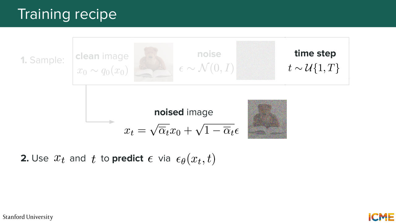
1:27:45 What you do is you take that noised image, you take the noise level, and then what you do
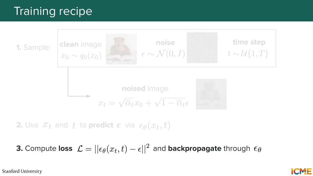
1:27:52 is you try to predict the noise that was added using your model, which right now we don't know. It's just a black box. And you compute the loss and you do your back propagation. So that's the training. And then the inference is you sample your noise,
1:28:14 which is super easy to do. And what you do is you go step by step from noise to less noise to less noise to less noise, up until arriving at t equals 0, which is clean image.

Shown briefly — discussed together with the adjacent slides.
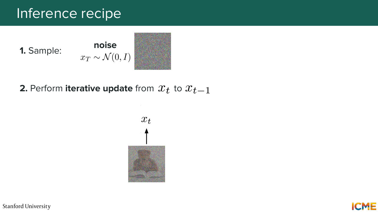
1:28:31 And here, what you do is you use the expression of p theta of xt minus 1 given xt, which is something we have derived, which is a function of the noisy image and the predicted noise that you can remove. And then you add some noise on top of it because let's remember that p theta of xt minus 1 given xt is a normal distribution. So the noise here just corresponds to the standard deviation of that distribution.
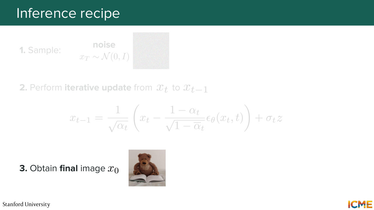
1:29:11 And when you do that from big T to 0, you then obtain your clean image. Cool. I know this was a lot. I know this is lecture 1. I can tell you that this lecture is probably the most difficult
1:29:27 of the eight first lectures. So if you feel a little bit like it's a lot to digest,
1:29:33 it's normal. Hopefully we've tried to make it a bit more digestible. Luckily, there is a recording.
1:29:38 We have the notes, we have everything. I mean, hopefully, if we don't, just let us know.
1:29:44 And with that, I'm going to give it to Shervin.
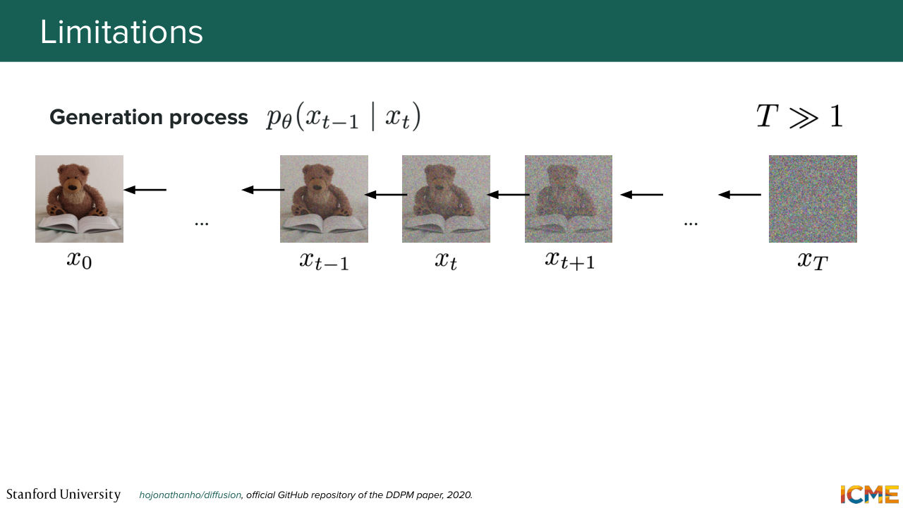
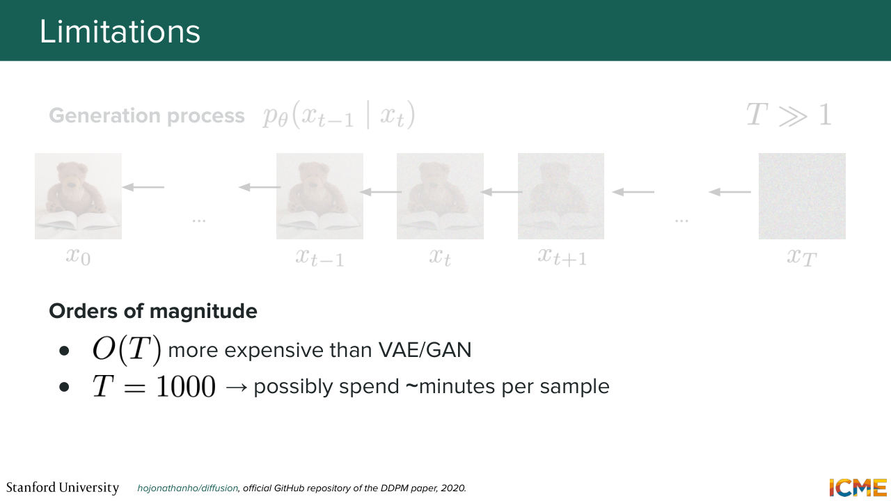
1:29:49 Thank you, Afshin. So now we saw how to generate a clean image starting from noise. And what we're seeing in this equation is that we need to repeat the same procedure big T times. And the thing is this big T is usually quite large. So it's the order of magnitude of 1,000, for example, in the original paper. And let's say you take the reference
1:30:23 point of existing image generation models before that, let's say VAEs or GANs, and you compute the amount of time
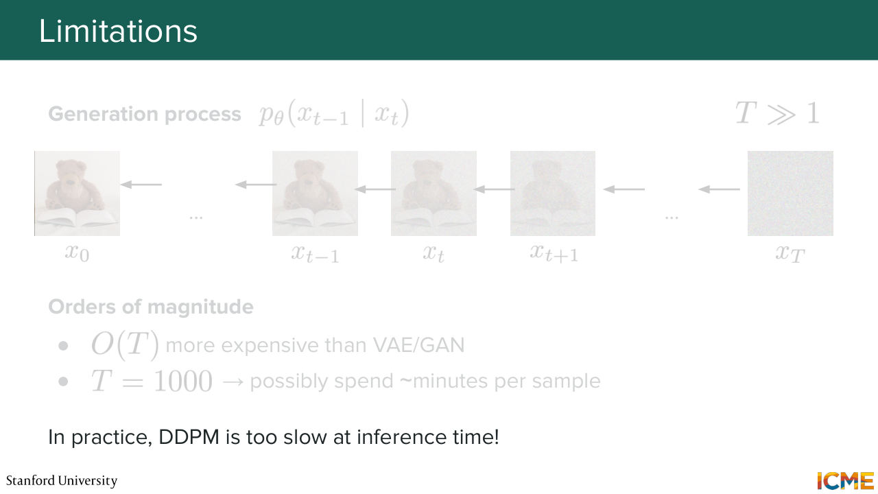
1:30:30 it takes to generate a single image, which is the forward pass. So you have to do that now t times. Let's say you had to do it for 100 milliseconds. Now it might take the order of magnitude of minutes, which is not great. So one comment that we have out of all of this is that we want to bring the computational burden down at inference time. So what can we do to make that happen?
1:30:58 So I will first show the equation that Afshin has shown, linking the generation process from step t, which is a denoiser image, to step t minus 1, which is the slightly cleaner image, which was defined by that generation process written on the slides.
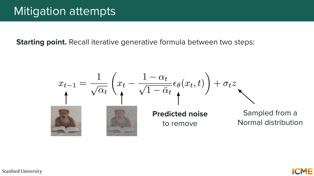
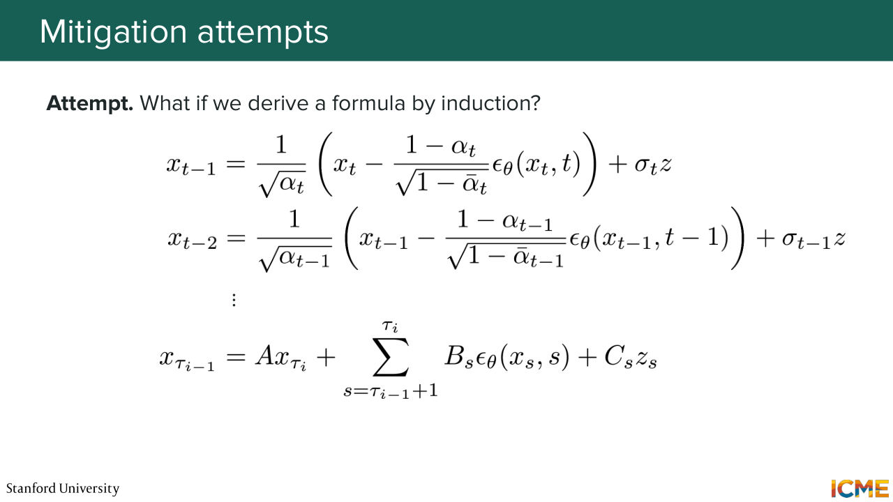
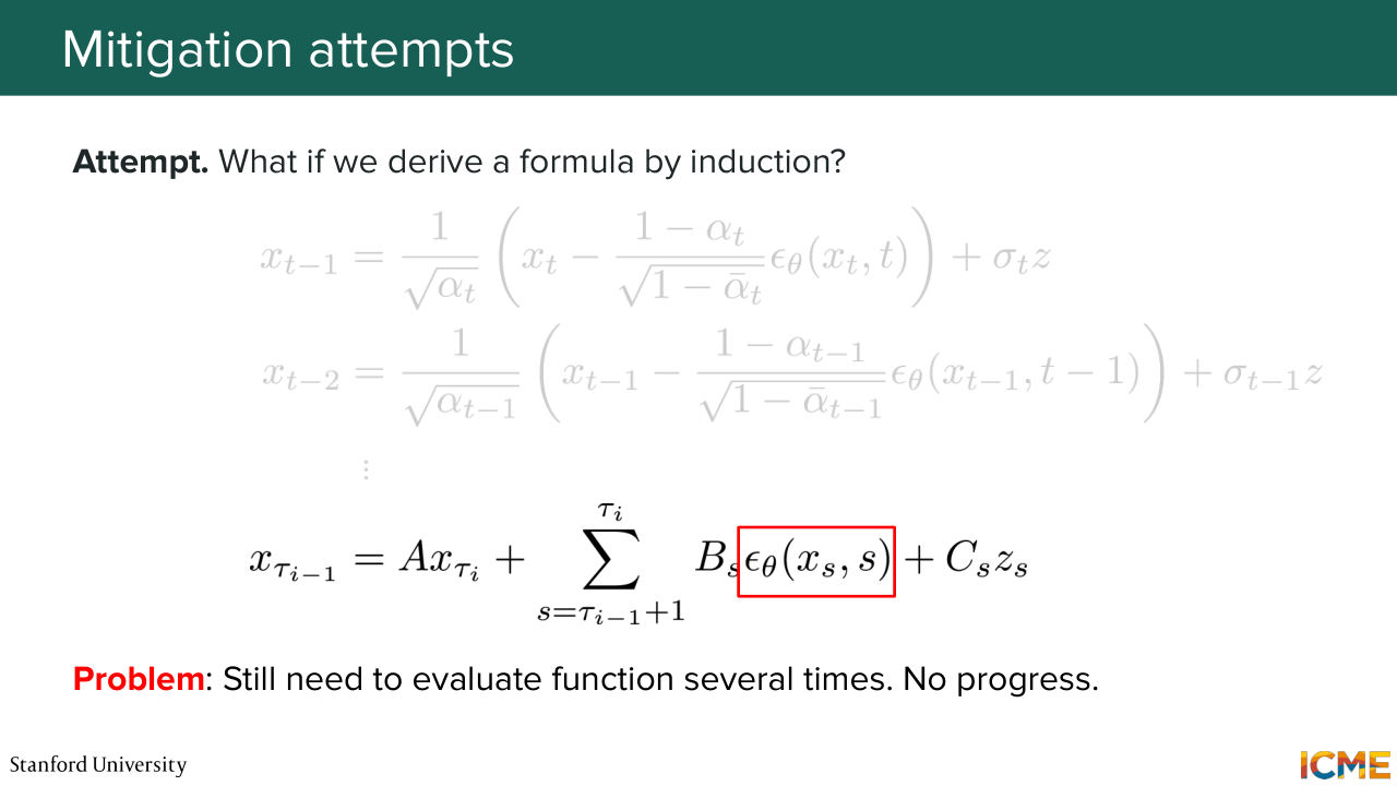
1:31:20 And we're going to try to see how to make these steps shorter. So what can we do? One strategy could be to try to skip steps. And the first thought that comes to mind is to write down equations and see if we can link a lower step to a higher one
1:31:46 and see if we can make a connection between the two without going through each of the steps. So let's start by writing down the same equation for step t minus 1, and then t minus 2, and so on. And you come up with a relationship linking a lower step that you index by some other sequence of numbers that you call tau I, which is a sequence of numbers between 0
1:32:16 and big T, where the gap between consecutive numbers is bigger than 1 potentially, and you end up with a relationship that involves step number tau I, which is the larger step number, and some sum over some numbers and some sampled noise. And as you can see, it hasn't brought us
1:32:44 very far because you still have quite a bit of model evaluations to make, which is exactly the gap between the two steps. So that didn't work. What can we do next? So let's just keep that sequence of numbers that represents sequences of steps that skip some in between.
1:33:10 One thing we could do is try to guess a formula that links two different steps. And I'm showing you one proposal of such a formula. And I'm not going to derive it, but just
1:33:24 going to verify that this makes sense for two consecutive steps. So if you say tau I is step t, and tau I minus 1
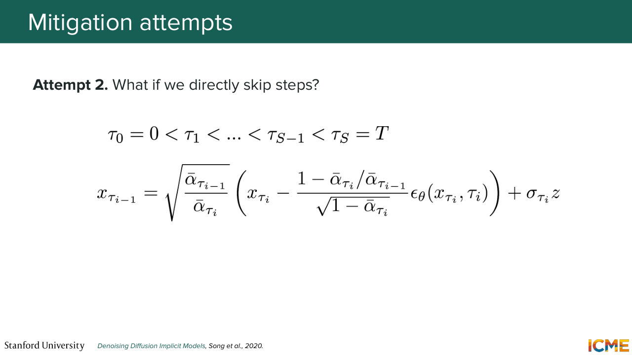
1:33:34 is step t minus 1, when you replace the numbers in there, you will find again the relationship between step t minus 1 and t. And so let's suppose you use such a relationship
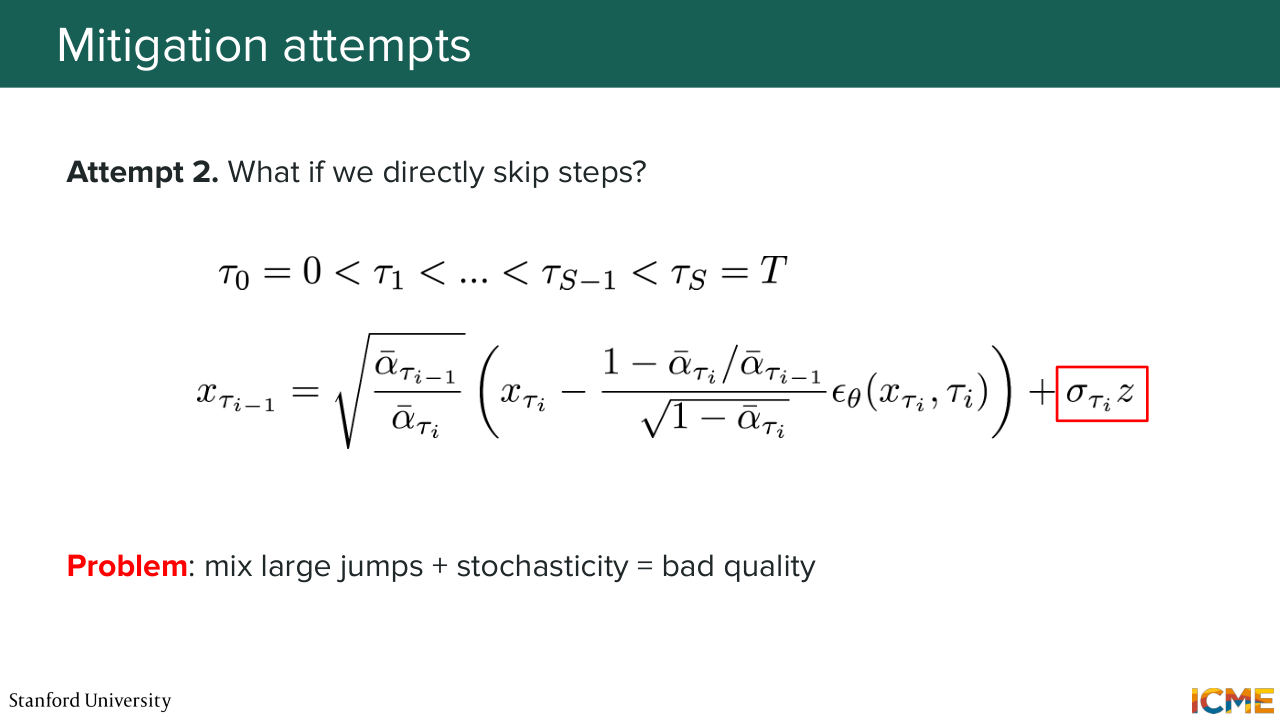
1:33:50 to link two different steps. Then what you realize in practice is that as the amount of stochasticity that you have within steps increases, then your quality is going to get worse as a function of the step size. So did that make sense. So by the way, the density of formulas in this last part is slightly higher than in the previous parts.
1:34:23 And the goal here is more to get the intuition of skipping steps and seeing how it works more than looking like at each formula separately. So does that make sense so far? OK, great. So now we have tried to skip steps and we have found a relationship that could link the two. But we see that the quality is not great when you take large step sizes.
1:34:55 So what you're trying to do now is trying to do this large step skipping, but avoid that level of stochasticity between steps.
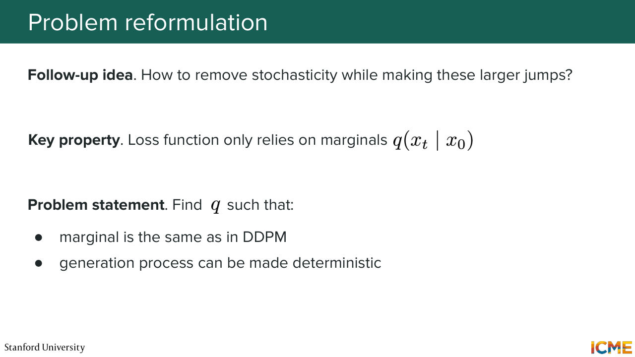
1:35:08 So in order to do so we go back to the drawing board and look at the derivation of the loss function that you had in the case of DDPM. And one thing we realize is that the a key part to get to the formulation of the DDPM loss was the marginal q of xt given x0.
1:35:33 And we realize that when we do modeling choices that reproduces that relationship on q, then you can have a model that is based on the same loss. So this is one observation. So the problem statement comes back to finding such a q that reproduces
1:36:02 these marginal probabilities. So with the same x of xt given x0. And the second constraint that we want to put ourselves is to have a generation process that forgoes of that stochasticity term in order to try to see if we can mitigate the fact that quality of generation gets worse. This is the problem statement. I'm going to write this down in more mathematical terms.
1:36:37 So we want to find a familiar function, let's say q sigma-- and I'm going to say what sigma is very soon and motivates why we are talking about the family function here-- such that we match the marginals with respect to the DDPM forward process. And the second condition where I said
1:37:03 that we don't want any stochasticity between two generation steps is translated by the fact that we want p theta of the least noisy image, given the noisy image to be deterministic,
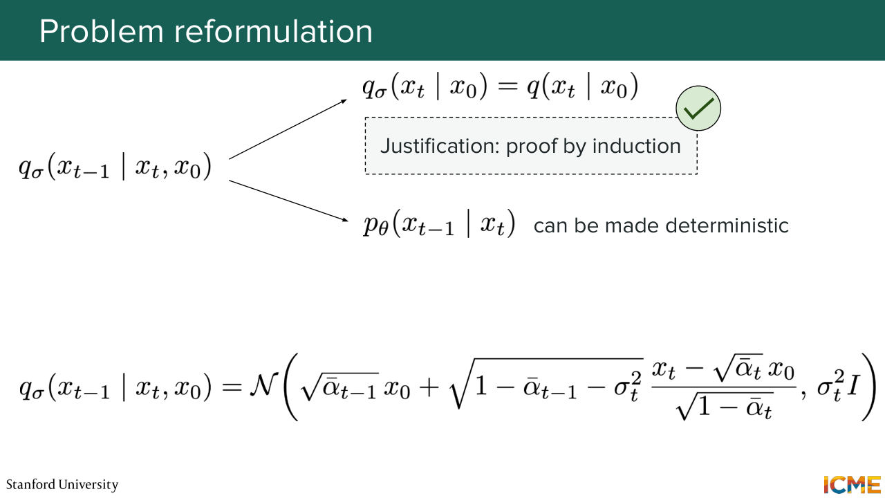
1:37:17 meaning that once you have xt, then your generation process gives you xt minus 1 as a one to one mapping,

1:37:25 so there is no more noise term. Does everyone agree on that? So I'm going to throw at you a formula and verify that this works. So this formula is parameterized by a parameter that is called sigma here that is a hyperparameter.
1:37:55 And by reasoning with the process of induction, we can verify that the marginals q sigma of xt given x0 matches the ones that we had in the case of DDPM. And when you set sigma to 0, you can
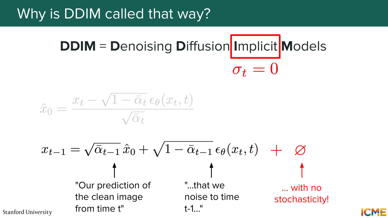
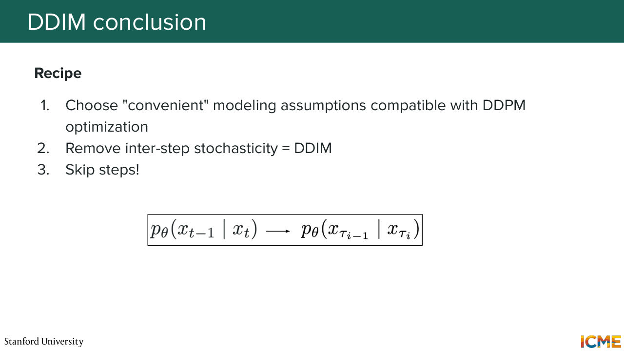
1:38:16 see that this term becomes just a mean with 0 variance. So you can link xt minus 1 to xt with no stochasticity. OK, great. And so this state of mind and coming to the realization that you have such a family of functions that verify that, and the fact that this is attractive to seek is part of this DDIM paper, where
1:38:51 the only term that changes with respect to the title of DDPM is this P, probabilistic, to I, implicit. So the probabilistic part of DPM translated the facts that when you generated a clean image out of noise, you had this probabilistic nature between two steps. But in this DDIM formulation where you don't have stochasticity at the generation step between two
1:39:20 consecutive steps, the stochastic part only comes when you sample your initial noise. So your xT. And this is why we call the diffusion process implicit because the probabilistic part is not something that you see between consecutive steps, but rather sets at the beginning of the generation process. So I think there was a question at the very beginning on why don't you start at the same point every time.
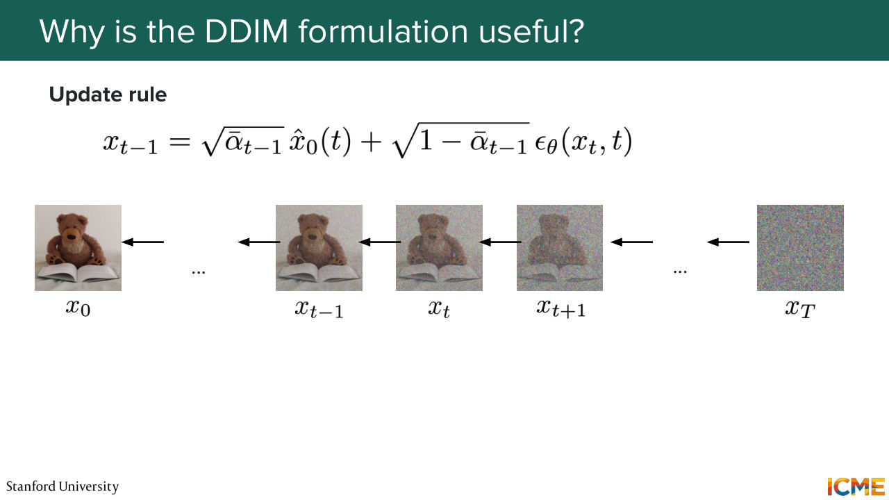
1:39:52 So if you were to do that, then DDIM wouldn't have worked because once you set your initial point of noise, then you determine deterministically your n image. And then in this case, one thing we can do is, at each step t, we can approximate our belief of what the clean image could
1:40:21 look like. So if you remember, the marginal distribution q of xt given x0 gives you a relationship between xt, x0, and the noise. And if you rearrange the terms, then you can approximate x0 at every step. This is just the rearrangement of terms that proves that. And then you can plug-in that approximation of x0
1:40:52 into the formula that we had just before to determine xt minus 1 by weighting this term accordingly and adding to it adequate noise weighted by the right coefficient at step t minus 1. And as you can notice here, there is no added stochasticity by construction of this family of forward processes Q sigma when sigma equals 0, which is the property that we
1:41:22 were after here. So does that make sense so far? So the question is where's the skipping steps here. We have not skipped any steps so far. We're just constructing the generation process. OK, great. So if you recall, you had these DDPM generation process
1:41:58 that you had that did not skip steps. So you had to go one step at a time. And now you can adapt the formula that we saw from step t
1:42:12 to step t minus 1. But now between these schedule of steps
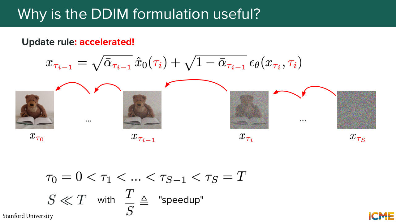
1:42:17 tau I's where at step tau I minus 1, you predict your best guess at what the clean image x0 is based

1:42:31 on your step tau I, and you approximate the noise that you need to remove. And you weigh each of these terms at the step tau I minus 1, which is how you get this formula. And here, we define some concepts. So when I talked about the sequence of steps tau I's, so the length of that sequence is s.
1:43:02 So we call it s. And t over s is the effective speedup. So instead of spending t steps to generate a new sample, you spend s steps. And with that in mind, the value for the speedup that people typically take is between 10 to 100.
1:43:26 And as you can guess, it doesn't come for free.
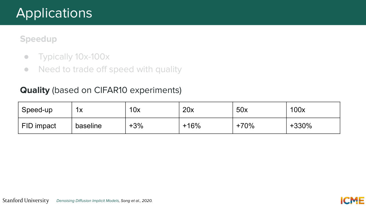
1:43:31 So it's a trade off between speed and actual quality that you get in the end. And the actual values that people take are more on the order of magnitude of 10 to 50. And here, I'm showing what the authors showed in one of their experiments, the evolution of one metric. So here, FID means Fréchet Inception Distance,
1:43:56 which is a metric that we'll cover in lecture 7 when we'll talk about evaluations.
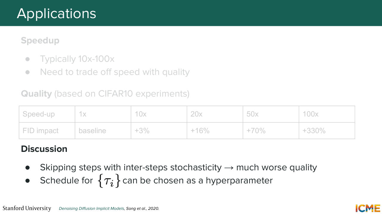
1:44:01 So now I'm not going to cover it in detail. Just going to tell you that it translates how the generated images look like. And so the absolute values don't necessarily mean much. But we can see the impact on quality based on relative differences. And you can see that you can speed up the process by taking s of size such that at that 20x, you're not too far from
1:44:31 the baseline of not skipping steps at all. So the discussion here is so we realized that when you skipped steps, the stochasticity that you had between two consecutive steps that the generation process turned out to generate worse estimates of what a lower
1:44:59 step would be, which is why removing it is better here. So here, we don't show the comparison with methods that do not remove the stochasticity, but the paper goes at length into showing that when you do have stochasticity, the results are much worse. So if I had to summarize the thought process that we went through, we looked at the DDPM loss,
1:45:28 we looked at the core ingredients of what got us there, which was q of xt given x0. We chose q sigma that verified the same relationship. And we made q sigma such that it could be made-- so we could have a generation process p theta that is deterministic. And once we had this deterministic generation
1:45:53 process, so we call it DDIM. And then we skip steps, and we get the transition from a generation process that needs to go through T steps

1:46:06 to one that only needs to go through S steps, which is what we got in the end. And with that, thank you very much for your attention and have a great weekend.